Chapter 5 Split&Merge Algorithms
Quicksorts (and Z:cksorts) have the following limitations
- they are not stable15
- they have \(\mathcal{O}(N^2)\) worst case
- their SWAPing limits to equally-sized elements
- their partitioning phase is difficult to parallelize
A generic sorting algorithm must deliver:
- stable positions with regard to ties
- a \(\mathcal{O}(N \log{N})\) worst case (deterministic)
- can be implemented with variable-sized elements
- can be implemented parallel in both, divide and conquer phases
Divide&Conquer generic-sorting can be done in the Split&Merge or in the Partition&Pool paradigm, I focus on Split&Merge algorithms here (generic Partition&Pool algorithms are considered in section Partition&Pool Algorithms).
innovation("Split&Merge","T*","Recursive split and merge paradigm")
dependency("Split&Merge","Divide&Conquer")
5.1 The Mergesort-Dilemma
Regarding binary Mergesort the prior art has basically four camps:
- balanced-Mergesort (using 100% buffer)
- natural-Mergesort (using not more than 50% buffer)
- Mergesort with block-managed memory (parsimoniously using \(\mathcal{O}(\sqrt(N))\) buffer)
- in-place-Mergesort (insisting on \(\mathcal{O}(1)\) or not more than \(\mathcal{O}(\log(N))\) buffer)
There is an inherent space-time trade-off: the less buffer required, the less speed achieved. There was lots of academic interest to find the perfect in-place-Mergesort (termed the “holy sorting grail” by Robert Sedgewick), however, in practice, in-place-Mergesorts were rarely used, because they were just too slow. Mergesort with block-managed memory requires a certain implementation complexity, hence is also not popular. For more information see the Low-Memory section. This leaves us with balanced-Mergesort versus natural-Mergesort.
In practice one finds many variations – often inefficient – of Mergesort. I consider the following two algorithms as prototypical for the most efficient algorithms of two camps:
5.2 First algo (Bimesort)
innovation("Bimesort","T","Nocopy mergesort with bitonic merge")
dependency("Bimesort","Split&Merge")
dependency("Bimesort", "Symmetric-sorting")
We need to combine certain teaching of the prior art to obtain a fair reference algorithm that represents the knowledge of the prior art, which requires a bit of your attention and patience. The first step towards the reference algorithm is the definition of Bimesort.
In chapter 12 (Mergesort) of Sedgewick (1990) taught on page 164 a Merge algorithm that uses two sentinels. This has the advantage that the inner loop does not need any explicit loop checks (stop conditions), but has the disadvantage that a suitable sentinel value needs to exist, needs to be known and allocated memory needs to reserve extra space for two sentinels, which is not practical in many settings. Hence, Sedgewick (1990) on page 166 taught a Mergesort that uses a Bitonic Merge which does not need sentinels, but still needs only one loop check The book does not mention, that the sort is not stable as a consequence from the fact that the merge is not stable. In a later version, Sedgewick (1998) still teaches the unstable Program 8.2 Abstract in-place-merge, but added an exercise that mentions missing stability and asks students to fix the merge. So far all the mentioned code needed two moves per element and recursion level for copying data from memory \(A\) to buffer \(B\) and merging back to \(A\). Sedgewick (1998) now teaches Program 8.4 Mergesort with no copying, an algorithm that alternates between merging from memory \(A\) to memory \(B\) one recursion level and merging from \(B\) to \(A\) on the next level, and hence saves the unnecessary copying. This is however not compatible with calling Program 8.2 Abstract in-place-merge with its two moves per element.
Sedgewick (page 346) mentions as a “superoptimization” the possibility to combine nocopy-Mergesort with a bitonic merge strategy: “We implement routines for both merge and mergesort, one each for putting arrays in increasing order and in decreasing order”. If one actually does this, even using truly stable merges for both orders, then the result is - again - an unstable algorithm, unless we replace the word “decreasing” in the above sentence with Ascending from Right (AscRight). I don’t know whether Sedgewick’s superoptimization was stable or not (the code is not in the book), but the key message here is: what Sedgewick calls a “mindbending recursive argument switchery … only recommended to experts”, turns into a precise instruction as soon as we use the the terms Ascending from Left (AscLeft) and AscRight. Within the greeNsort® definition of Symmetric-sorting stability is easy, the resulting algorithm I call Bimesort. We show it here for its elegance, in a simplified version without register caching and without insertion-sort tuning. For this paper Split&Merge algorithms are implemented in C with pointers, the implementation assumes the data in \(A\), an equally large buffer \(B\) and the data needs to be copied from \(A\) to \(B\) before sorting, although this is not needed for certain recursion depths. Note that all the complexity of duplicating the merge- and recursive sort-function comes with a severe disadvantage: the algorithm must move the data on each recursion level, even if the data is perfectly presorted.
void Bmerge_AscLeft(ValueT *z, ValueT *l, ValueT *m, ValueT *r){
  while(l<=m){
    if (LT(*r,*l)){
      *(z++) = *(r--);
    }else{
      *(z++) = *(l++);
    }
  }
  while(m<r){
    *(z++) = *(r--);
  }
}
void Bmerge_AscRight(ValueT *z, ValueT *l, ValueT *m, ValueT *r){
  while(m<r){
    if (LT(*r,*l)){
      *(z++) = *(l++);
    }else{
      *(z++) = *(r--);
    }
  }
  while(l<=m){
    *(z++) = *(l++);
  }
}
void Bsort_AscLeft(ValueT *a, ValueT *b, IndexT n){
IndexT m;
if (n>1){
m = n/2;
Bsort_AscLeft(b, a, m);
Bsort_AscRight(b+m, a+m, n-m);
Bmerge_AscLeft(a, b, b+m-1, b+n-1);
}
}
void Bsort_AscRight(ValueT *a, ValueT *b, IndexT n){
IndexT m;
if (n>1){
m = n/2;
Bsort_AscRight(b, a, m);
Bsort_AscLeft(b+m, a+m, n-m);
Bmerge_AscRight(a, b, b+m-1, b+n-1);
}
}5.3 Reference algo (Knuthsort)
innovation("Knuthsort","T","Nocopy mergesort with Knuth's merge")
dependency("Knuthsort","Split&Merge")
All of Sedgwicks’s effort about his bitonic merge-strategy ignored an earlier teaching of D. Knuth (1973), that you can have one loop check much easier: only that input sequence from which the last element has been taken for the merge can exhaust, hence only that one needs to be checked! Furthermore Katajainen and Träff (1997) has taught how to get away with even a half expected loop check. Katajainen’s clever merge qualifies as ‘tuning’ because it costs an extra key-comparison at the beginning for identifying which of the two input sequences will exhaust first, only this one needs to be checked, about 50% in a balanced merge. But Knuth’s clever merge can be seen as a basic algorithmic technique without such a trade-off. It can easily be combined with Sedgwicks’s Nocopy-Mergesort. To honor Programming-Artist Donald Knuth, I call this Knuthsort. It is much simpler than Bimesort and serves as the main prior art reference for the greeNsort® algorithms. Here is the code in a simplified version without register caching and without insertion-sort tuning:
void Kmerge(ValueT *z, ValueT *l, ValueT *m, ValueT *r){
  ValueT *j=m+1;
  for (;;){
    if (LT(*j, *l)){
      *(z++) = *(j++);
      if (j > r)  // one check either here
        break;
    }else{
      *(z++) = *(l++);
      if (l > m)  // or one   check here
        break;
    }
  }
  while(l <= m)
    *(z++) = *(l++);
  while(j <= r)
    *(z++) = *(j++);
}
void Ksort(ValueT *a, ValueT *b, IndexT n){
IndexT m;
if (n>1){
m = n/2;
Ksort(b, a, m);
Ksort(b+m, a+m, n-m);
Kmerge(a, b, b+m-1, b+n-1);
}
}
Figure 5.1: Knuthsort compared to Knuthsort. The left chart compares the absolute energy consumed for 8 input patterns and the TOTAL (of 5). The right chart shows the respective ratios to the median of the reference algorithm (here Knuthsort). The red lines show the reference medians.
| %M | rT | pcdE | pcdF | |
|---|---|---|---|---|
| TOTAL | 2 | 0.0937272 | 1.2240148 | 2.4480297 |
| ascall | 2 | 0.0224867 | 0.3337648 | 0.6675297 |
| descall | 2 | 0.0635693 | 0.8502343 | 1.7004686 |
| ascglobal | 2 | 0.0896020 | 1.1903291 | 2.3806582 |
| descglobal | 2 | 0.0877766 | 1.1275486 | 2.2550973 |
| asclocal | 2 | 0.0976911 | 1.2881909 | 2.5763818 |
| desclocal | 2 | 0.1405737 | 1.8402222 | 3.6804445 |
| tielog2 | 2 | 0.0712948 | 0.9417672 | 1.8835344 |
| permut | 2 | 0.1640641 | 2.1191219 | 4.2382439 |
5.4 2nd Reference (Timsort)
T. Peters (2002) Timsort is famous for its \(\mathcal{O}(N)\) best-case for presorted data, but it comes with the following limitations:
- it uses an inefficient merge which needs two moves per element (compared to one move per element in Knuthsort)
- it is inherently serial
- it invests extra-operations (“galloping-mode”) to speed-up best-cases (which violates the T-level technique – (DO) (NO)t (TU)ne the (BE)st case (DONOTUBE) principle)
Since the the python implementation is for lists only and cannot compete with greeNsort®, and since a fair re-implementation would have been too complicated, the test-bed uses as a reference the C++ implementation of Timothy Van Slyke from 2018, the most competitive implementation I could find.16. Here some data on Timsort, the magenta lines show the eFootprint medians17 projected onto the Energy scale (calculated as \(Energy_{Knuthsort} \cdot \%RAM_{Knuthsort} / \%RAM_{Timsort}\)).

Figure 5.2: Timsort compared to Knuthsort. The left chart compares the absolute energy consumed for 8 input patterns and the TOTAL (of 5). The right chart shows the respective ratios to the median of the reference algorithm (here Knuthsort). The red/magenta lines show the Energy/eFootprint reference medians.
| r(%M) | r(rT) | r(pcdE) | r(pcdF) | d(pcdE) | p(rT) | p(pcdE) | p(pcdF) | |
|---|---|---|---|---|---|---|---|---|
| TOTAL | 0.75 | 0.98 | 0.99 | 0.75 | -0.01 | 0.0000 | 0.0076 | 0 |
| ascall | 0.75 | 0.09 | 0.09 | 0.07 | -0.30 | 0.0000 | 0.0000 | 0 |
| descall | 0.75 | 0.05 | 0.05 | 0.04 | -0.80 | 0.0000 | 0.0000 | 0 |
| ascglobal | 0.75 | 1.01 | 0.97 | 0.72 | -0.04 | 0.0786 | 0.0002 | 0 |
| descglobal | 0.75 | 1.24 | 1.24 | 0.93 | 0.27 | 0.0000 | 0.0000 | 0 |
| asclocal | 0.75 | 1.21 | 1.25 | 0.94 | 0.32 | 0.0000 | 0.0000 | 0 |
| desclocal | 0.75 | 0.83 | 0.85 | 0.64 | -0.28 | 0.0000 | 0.0000 | 0 |
| tielog2 | 0.75 | 1.21 | 1.17 | 0.88 | 0.16 | 0.0000 | 0.0000 | 0 |
| permut | 0.75 | 1.27 | 1.31 | 0.98 | 0.66 | 0.0000 | 0.0000 | 0 |
The TOTAL data show that Timsort is not much better than Knuthsort on the RUNtime and pcdEnergy KPIs: The improvements for presorted data are offset by deterioration for heavy sorting tasks. On the pcdFootprint KPI is is much better, because it requires only 75% memory.
5.5 Pre-Adpative (Omitsort)
innovation("Data-driven-location","B","data decides return memory")
innovation("Omitsort","A","skip merge and return pointer to data")
dependency("Omitsort", "Data-driven-location")
dependency("Omitsort","Split&Merge")
I now disclose how to modify Knuthsort to be adaptive for presorted data: differing from the prior art greeNsort® gives-up control over the location of the merged-data. If the two input sequences are not overlapping and merging is not needed, then it is possible to simply omit merging and the data stays where it was. The recursive function returns in which of the two memory areas the data resides. I call this method Data-driven-location and the resulting Omitsort has the following properties:
- like Knuthsort it uses 100% buffer (unlike Timsort which needs not more than 50%)
- unlike Knuthsort it does not require redundant upfront copying from data to buffer
- like Knuthsort and unlike Timsort it uses an efficient merge which needs only one move per element
- unlike Knuthsort and like Timsort for perfectly presorted branches no elements will be moved
- like Timsort, Omitsort has a \(\mathcal{O}(N)\) best-case: due to not more than \(N\) non-overlap checks (and no moves)
- like Knuthsort and unlike Timsort a fully parallel implementation is possible

Figure 5.3: Omitsort compared to Knuthsort
| r(%M) | r(rT) | r(pcdE) | r(pcdF) | d(pcdE) | p(rT) | p(pcdE) | p(pcdF) | |
|---|---|---|---|---|---|---|---|---|
| TOTAL | 1 | 0.97 | 0.97 | 0.97 | -0.04 | 0.0000 | 0.0000 | 0.0000 |
| ascall | 1 | 0.11 | 0.12 | 0.12 | -0.29 | 0.0000 | 0.0000 | 0.0000 |
| descall | 1 | 0.98 | 0.99 | 0.99 | -0.01 | 0.0000 | 0.0015 | 0.0015 |
| ascglobal | 1 | 1.00 | 0.98 | 0.98 | -0.02 | 0.0015 | 0.1706 | 0.1706 |
| descglobal | 1 | 1.00 | 1.01 | 1.01 | 0.02 | 0.4777 | 0.0374 | 0.0374 |
| asclocal | 1 | 1.07 | 1.07 | 1.07 | 0.09 | 0.0000 | 0.0000 | 0.0000 |
| desclocal | 1 | 0.99 | 0.99 | 0.99 | -0.02 | 0.0001 | 0.0000 | 0.0000 |
| tielog2 | 1 | 0.99 | 0.99 | 0.99 | -0.01 | 0.0000 | 0.1050 | 0.1050 |
| permut | 1 | 1.00 | 1.00 | 1.00 | 0.00 | 0.8920 | 0.6938 | 0.6938 |
Compared to Knuthsort, Omitsort needs only about 97% Energy, for presorted data it is 12%.
5.6 Bi-adpative (Octosort)
innovation("Undirected-sorting","C","not requesting asc/desc order")
innovation("Data-driven-order","B","data decides asc/desc order")
innovation("Octosort","A","lazy directed undirected sort")
dependency("Data-driven-order", "Undirected-sorting")
dependency("Octosort", "Data-driven-location")
dependency("Octosort", "Data-driven-order")
Omitsort still has a limitation: it is adaptive to presorted (e.g. left-ascending) but not to reverse-sorted (e.g. left-descending) data. If the data is left-descending, then sorting incurs \(\mathcal{O}(N \log{N})\) moves (and depending on implementation details also comparisons). But if a reversed Omitsort had been used which sorts left-descending, the caller could reverse the final descending sequence with not more than \(N\) moves (and \(N\) comparisons for stability), which would still be a \(\mathcal{O}(N)\) best-case. What to do without upfront knowledge that the data was descending from left?
I now disclose how to modify Omitsort to be adaptive for presorted and reverse-sorted data: I drop the prior art assumption that the sorting order needs to be specified in the API to the recursive function. It is possible to let the recursive function decide whether to sort or to reverse-sort and only lazily enforce the desired order. After the recursion is finished, the obtained order can be returned (undirected API) or the desired order can be forced (directed API). I call this Data-driven-order and the resulting Octosort has the following properties:
- like Omitsort, the presorted best-case costs less than \(N\) comparisons (and no moves)
- unlike Omitsort, the reverse-sorted best-case costs less than \(2N\) comparisons and \(N\) moves
- like Timsort, the best-case is \(\mathcal{O}(N)\) for presorted and reverse-sorted data

Figure 5.4: Octosort compared to Knuthsort
| r(%M) | r(rT) | r(pcdE) | r(pcdF) | d(pcdE) | p(rT) | p(pcdE) | p(pcdF) | |
|---|---|---|---|---|---|---|---|---|
| TOTAL | 1 | 0.88 | 0.89 | 0.89 | -0.14 | 0 | 0 | 0 |
| ascall | 1 | 0.14 | 0.13 | 0.13 | -0.29 | 0 | 0 | 0 |
| descall | 1 | 0.07 | 0.07 | 0.07 | -0.79 | 0 | 0 | 0 |
| ascglobal | 1 | 1.04 | 1.04 | 1.04 | 0.05 | 0 | 0 | 0 |
| descglobal | 1 | 1.07 | 1.08 | 1.08 | 0.09 | 0 | 0 | 0 |
| asclocal | 1 | 1.10 | 1.12 | 1.12 | 0.15 | 0 | 0 | 0 |
| desclocal | 1 | 0.72 | 0.72 | 0.72 | -0.51 | 0 | 0 | 0 |
| tielog2 | 1 | 1.08 | 1.10 | 1.10 | 0.09 | 0 | 0 | 0 |
| permut | 1 | 1.07 | 1.07 | 1.07 | 0.15 | 0 | 0 | 0 |
Compared to Knuthsort, Octosort needs only about 90% Energy, for presorted and reverse-sorted data it is 14% and 7%.
5.7 Gapped-merging (GKnuthsort)
innovation("Gapped-setup","B","odd-even data-buffer layout")
dependency("Gapped-setup", "Ordinal-machine")
innovation("Gapped-merging","B","merge in odd-even data-buffer layout")
dependency("Gapped-merging", "Gapped-setup")
innovation("GKnuthsort","A","Knuthsort in odd-even data-buffer")
dependency("GKnuthsort", "Gapped-merging")
dependency("GKnuthsort", "Knuthsort")
Now I address a more fundamental problem of the prior art Split&Merge algorithms: they move the data always between two distant memory regions \(A\) and \(B\). Even if \(A\) and \(B\) are contiguous neighbors, the minimum distance of the \(\mathcal{O}(N\log{N})\) moves is \(N\). This differs dramatically from the distance-behavior of Quicksorts. The prior art knows that Quicksorts are cache-friendly, but it underappreciates that Quicksorts are distance-friendly: Quicksort recursion zooms into local memory such that the maximum distance is the current local size \(n\) of the problem (and not the global problem-size \(N\)).
Now I drop one prior art assumption behind those prior art Split&Merge algorithms: that data and buffer are separate memory regions. One way to make Split&Merge algorithms more distance-friendly is to define \(A\) and \(B\) as odd and even positions in contiguous memory. Doing so gives a local problem size \(2n\). Adapting Knuthsort to Gapped-merging gives GKnuthsort:
| position | 1 | 2 | 3 | 4 | 5 | 6 | 7 | 8 |
|---|---|---|---|---|---|---|---|---|
| setup | 4 | . | 3 | . | 2 | . | 1 | . |
| merge | . | 3 | . | 4 | . | 1 | . | 2 |
| merge | 1 | . | 2 | . | 3 | . | 4 | . |
However, this approach has the following shortcomings
- elements to be sorted must have equal size
- it is not fast on current hardware
Speed might be improved by using odd and even blocks of data and buffer, say of size 1024. However, I will develop this idea into a more interesting direction.
5.8 Buffer-merging (TKnuthsort, Crocosort)
innovation("Buffer-merging","B","merging data and buffer")
innovation("Buffer-splitting","B","splitting data and buffer")
dependency("Buffer-merging","Split&Merge")
dependency("Buffer-splitting","Split&Merge")
dependency("Buffer-merging","Gapped-setup")
innovation("TKnuthsort","A","Knuthsort with buffer-merging (T-moves)")
dependency("TKnuthsort", "Buffer-merging")
dependency("TKnuthsort", "GKnuthsort")
innovation("Crocosort","A","Knuthsort with buffer-merging (R-moves)")
dependency("Crocosort", "Buffer-merging")
dependency("Crocosort", "GKnuthsort")
Now I drop a prior art assumption behind prior art Split&Merge algorithms: they focus on merging the data, but not the buffer. greeNsort® treats the buffer like the data as a first-class objective of merging. Merging must split and merge data and buffer, then bigger and bigger contiguous regions of data and of buffer are obtained as the merging proceeds.
A naive way of merging data and buffer is self-recursion which maintains an invariant data-buffer pattern, for example placing data left and buffer right within local memory. After a gapped setup, in order to maintain this pattern, data must first be transferred to one half of the memory and then merged to the other (TKnuthsort):
| position | 1 | 2 | 3 | 4 | 5 | 6 | 7 | 8 |
|---|---|---|---|---|---|---|---|---|
| setup | 4 | . | 3 | . | 2 | . | 1 | . |
| transfer | . | . | 4 | 3 | . | . | 2 | 1 |
| merge | 3 | 4 | . | . | 1 | 2 | . | . |
| transfer | . | . | . | . | 3 | 4 | 1 | 2 |
| merge | 1 | 2 | 3 | 4 | . | . | . | . |
This can be somewhat optimized to not transfer all data, but only that data which is in the target half for merging. With a little care to not ruin stability, Crocosort gets away with only 50% relocation:
| position | 1 | 2 | 3 | 4 | 5 | 6 | 7 | 8 |
|---|---|---|---|---|---|---|---|---|
| setup | 1 | . | 2 | . | 3 | . | 4 | . |
| relocate | . | . | 2 | 1 | . | . | 4 | 3 |
| merge | 1 | 2 | . | . | 3 | 4 | . | . |
| relocate | . | . | . | . | 3 | 4 | 1 | 2 |
| merge | 1 | 2 | 3 | 4 | . | . | . | . |
However, on current CPUs, also the extra 50% relocation moves are too expensive and are slower than simple Knuthsort. What to do?
5.9 Symmetric-language method
innovation("Symmetric-language","B","symmetric semi-in-place merging data and buffer")
dependency("Symmetric-language", "Buffer-merging")
dependency("Symmetric-language", "Symmetric-sorting")
dependency("Symmetric-language", "Symmetric-recursion")
dependency("Symmetric-language", "Footprint")
Now I disclose the solution to distance-reducing data- and buffer-merging: instead of self-recursion, Symmetric-merging uses Symmetric-recursion over Buffer-asymmetry, where the left branch sorts ‘to left’ (i.e. data left, buffer right) and the right branch sorts ‘to right’ (i.e. data right, buffer left). As a result, the two buffer regions border each other and form one contiguous buffer space without requiring any extra moves.
Figure 5.5: Symmetric-language
The following is a description for symmetric Divide&Conquer, i.e. Split&Merge as well as Partition&Pool:
Let \(LB\) denote a buffer-asymmetric chunk of memory with data left and buffer right and let \(BR\) denote a buffer-asymmetric chunk with data right and buffer left. Then a symmetric pair of left and right chunks \(LBBR\) have a joint contiguous buffer memory \(BB\) in the middle and can be conquered either to the left into a bigger \(LLBB\)- chunk (which replicates the structure of the \(LB\)-chunk) or to the right to a bigger \(BBRR\)-chunk (which replicates the structure of the \(BR\)-chunk). Now consider a pair of such \(LBBR\) pairs \(LBBRLBBR\), and divide and conquer the left pair to the left and the right pair to the right to obtain \(LLBBBBRR\) (which replicates the structure of \(LBBR\) with a contiguous inner buffer area) and hence can be conquered again to the left or the right.
This recursive symmetric asymmetric data structure can be exploited with two flip-recursive merging functions toLeft() resp. toRight() that divide their \(LLBB\) resp. \(BBRR\) input into two smaller chunks \(LB\) and \(BR\), call toLeft() on \(LB\) and toRight() on \(BR\) and then conquer them to \(LLBB\) resp. \(BBRR\). toLeft() reads and writes the data in \(LBBR\) from right-to-left, toRight() reads and writes the data in \(LBBR\) from left-to-right.
It is understood that the recursive functions toLeft() and toRight() are designed to not further divide if the input chunk is small enough; as a stopping criterion I contemplate a chunk that contains only a single element (and hence the chunk is sorted), or I contemplate a greater limit to the size of the chunk, at which the recursive function calls a different function to sort the elements in the chunk (for example tuning with Insertionsort). It is understood that by calling toLeft() or toRight() on a suitable top-level chunk the data in that chunk gets finally sorted and that data and buffer both are returned in a contiguous memory area, although during recursion many chunks and hence many gaps existed. It is understood that the real sorting work of \(\mathcal{O}(N \cdot log{N})\) comparing and moving is done in the merging (or partitioning phases), while the splitting (or pooling) phases do not require more than \(O{N}\) moves (and obviously no comparisons). Here is a simple example for merging four keys using four buffer elements:
| position | 1 | 2 | 3 | 4 | 5 | 6 | 7 | 8 |
|---|---|---|---|---|---|---|---|---|
| setup to | L | B | B | R | L | B | B | R |
| setup do | 4 | . | . | 3 | 2 | . | . | 1 |
| merge to | L | L | B | B | B | B | R | R |
| merge do | 3 | 4 | . | . | . | . | 1 | 2 |
| merge to | L | L | L | L | B | B | B | B |
| merge do | 1 | 2 | 3 | 4 | . | . | . | . |
Now I generalize: symmetric merging needs no more than 50% buffer space. Let \(I\) denote ‘inner’ and \(O\) denote ‘outer’ and write \(LBBRLBBR\) as \(OBBIIBB\). As before \(OBBI\) is merged to the left and \(IBBO\) is merged to the right, hence both are merged (read and written) from inner to outer. Note that the outer data ought have the target order of sorting, for example ascending. Reading the inner and outer data starts from the innermost positions of \(I\) and \(O\) and proceeds to the outermost positions; and writing starts in \(BB\) at position \(|I| + |O|\) relative to the outermost position of \(O\). The merge is completed once the inner data is exhausted, the rest of the outer data is already in-place. The minimum size of \(BB\) is hence that of \(I\), hence required is \(|BB| \ge |I|\). If the splitting in symmetric Split&Merge is done such that the size of \(I\) is smaller or equal to the size of \(O\), hence required is \(|I| \le |O|\), it follows that a buffer size of \(I\) is sufficient. For a balanced split where \(|I| = |O|\) this amounts to 50% buffer. To better represent the relative sizes we may write \(B\) instead of \(BB\), and hence \(OBI\) (or \(IBO\)) for two chunks before merging to outer, where \(|I| \le |O|\) and \(|I| = |B|\).
| position | 1 | 2 | 3 | 4 | 5 | 6 |
|---|---|---|---|---|---|---|
| setup to | L | B | R | L | B | R |
| setup do | 4 | . | 3 | 2 | . | 1 |
| merge to | L | L | B | B | R | R |
| merge do | 3 | 4 | . | . | 1 | 2 |
| merge to | L | L | L | L | B | B |
| merge do | 1 | 2 | 3 | 4 | . | . |
Now recap the benefits of Symmetric-merging
- unlike GKnuthsort it operates on contiguous data
- like Knuthsort if is fully generic (stable, \(\mathcal{O}(N \log{N})\), allows variable size, allows parallelization)
- like Knuthsort (and Sedgewick’s Nocopy-mergesort) there are no unneeded moves and can be tuned
- but it needs not more than 50% buffer (where Knuthsort needs 100%)
- unlike Knuthsort it zooms into local memory and minimizes distances (similar to Quicksorts and Z:cksorts)
5.10 Frogsort & Geckosort
innovation("Frogsort","B","symmetric-merging ½-adaptive presorting")
dependency("Frogsort","Symmetric-language")
dependency("Frogsort","Buffer-splitting")
innovation("Geckosort","B","symmetric-merging ¼-adaptive pre/rev")
dependency("Geckosort","Symmetric-language")
dependency("Geckosort","Buffer-splitting")
Now let’s take a closer look at the Symmetric-merging. There are two algorithms to be distinguished, that I have named Frogsort and Geckosort, note that both names contain acronyms: (F)lip (R)ecursive (O)rganized (G)aps (FROG) and (G)ap (E)xchange (C)an (K)eep (O)rder (GECKO). In Frogsort the sorting order in both branches is the same, for example AscLeft:

Figure 5.6: Frogsort merges to left and to right (here AscLeft)
Note that Frogsort is automatically adaptive to pre-sorted data: the outer sequence remains in place, only the inner sequence is compared and moved. Once the inner sequence is moved, merging stops. This means that the cost of merging reduces from \(N\) comparisons and moves to \(N/2\) comparisons and moves. By investing an extra comparison to identify non-overlap, the \(N/2\) comparisons can also be saved. Hence Frogsort has yet another asymmetry: Order-asymmetry regarding adaptivity. There is an alternative to Frogsort.
Geckosort uses in the right branch the flipped order of the left branch:

Figure 5.7: Geckosort merges to left and to right (here Ascending)
As an example here follows the beautifully symmetric code forGeckosort1 in a simplified version without register caching and without insertion-sort tuning (full explanation in section Engineering Frogsort1):
void Geckomerge_toright_ascleft(
  ValueT *x
, ValueT *ll, ValueT *lr
, ValueT *rl, ValueT *rr
){
  for(;;){
    if (LT(*rl,*lr)){
      *(x++) = *rl++;
      if (rl>rr) break;
    }else{
      *(x++) = *lr--;
      if (ll>lr) return;
    }
  }
  while(ll<=lr){
    *(x++) = *lr--;
  }
  return;
}
void Geckomerge_toleft_ascright(
    ValueT *x
  , ValueT *ll, ValueT *lr
  , ValueT *rl, ValueT *rr
){
  for(;;){
    if (LT(*rl,*lr)){
      *(x--) = *rl++;
      if (rl>rr) return;
    }else{
      *(x--) = *lr--;
      if (ll>lr) break;
    }
  }
  while(rl<=rr){
    *(x--) = *rl++;
  }
  return;
}
void Geckoinit1_toleft_ascright(
ValueT *x , ValueT *y
, IndexT n, IndexT l, IndexT L
){
IndexT nr;
if (n <= 2){
if (n == 2){
ValueT t;
if (LE(x[l], x[l+1])){
t = x[l+1]; y[L+1] = x[l]; y[L] = t; // no in-place overwrite
}else{
y[L+1] = x[l+1]; y[L] = x[l];
}
}else{
y[L] = x[l];
}
}else{
nr = n / 2;
Geckoinit1_toleft_ascright(x, y, n - nr, l , L );
Geckoinit1_toright_ascleft(x, y, nr , l+n-1, L+n+nr-1);
}
}
void Geckoinit1_toright_ascleft(
ValueT *x, ValueT *y
, IndexT n, IndexT r, IndexT R
){
IndexT nl; ValueT t;
if (n <= 2){
if (n == 2){
if (GT(x[r-1], x[r])){
t = x[r-1]; y[R-1] = x[r]; y[R] = t; // no in-place overwrite
}else{
y[R-1] = x[r-1]; y[R] = x[r];
}
}else{
y[R] = x[r];
}
}else{
nl = n / 2;
Geckoinit1_toleft_ascright(x, y, nl , r-n+1, R-n-nl+1);
Geckoinit1_toright_ascleft(x, y, n - nl, r , R );
}
}void Geckosort1_toleft_ascright(
ValueT *y
, IndexT n
, IndexT L
){
if (n > 2){
IndexT nr = n / 2;
Geckosort1_toleft_ascright (y, n - nr, L );
Geckosort1_toright_ascleft(y, nr , L+n+nr-1);
Geckomerge_toleft_ascright(y+L+n-1, y+L, y+(L+(n-nr)-1), y+(L+n), y+(L+n+nr-1));
}
}
void Geckosort1_toright_ascleft(
ValueT *y
, IndexT n
, IndexT R
){
if (n > 2){
IndexT nl = n / 2;
Geckosort1_toleft_ascright(y, nl , R-n-nl+1);
Geckosort1_toright_ascleft(y, n - nl, R );
Geckomerge_toright_ascleft(y+R-n+1, y+(R-n-nl+1), y+(R-n), y+(R-(n-nl)+1), y+R);
}
}Note that Geckosort is as stable as Frogsort. Note further, that Geckosort is more symmetric than Frogsort: one branch is adaptive to pre-sorting, the other branch is adaptive to reverse-sorted data. This is reflected in the naming: Frogs are asymmetric regarding locomotion: the back legs of the frog are stronger than its front legs, this helps jumping forward. The Gecko is more symmetric with equally strong back and front legs, which supports his preferred hunting technique of invisibly slow sneaking up on the prey. Note finally, that Geckosort is not fully symmetric, because ties are considered presorted in one branch, and must be reversed in the other. Let’s recap the adaptivity implications of Symmetric-merging. Frogsort and Geckosort have four benefits over Bimesort and Knuthsort:
- they need not more (rather less) than 50% buffer compared to 100% in the prior art
- Symmetric-language reduces distances by zooming into local memory
- Symmetric-language needs only half the cost for presorted data (without any tuning)
- there is a choice between half-adaptivity for one order in Frogsort and quarter-adaptivity for both orders in Geckosort
These benefits come at minor costs and limitations:
- the code is more complex (albeit with symmetric redundancy that can be exploited in formal Code-mirroring)
- a \(\mathcal{O}(N)\) setup-phase is needed to distribute data with buffer gaps (Gapped-setup)
- like Bimesort but unlike Knuthsort even for perfectly presorted data, half of the elements must be moved, hence the cost remains \(\mathcal{O}(N\log{N})\) and cannot be tuned to \(\mathcal{O}(N)\) as was possible for Knuthsort with Omitsort and Octosort.
Now lets look at several ways to actually implement Frogsort (similar possibilities exist for Geckosort).
5.10.1 Engineering Frogsort0
innovation("Frogsort0","A","Frogsort on triplets or bigger chunks")
dependency("Frogsort0","Frogsort")
Frogsort0 Divides&Conquers triplets of memory cells: two cells contain two elements and a third empty buffer cell in the middle. The buffer in the middle allows to save one move for presorted data. The initial setup of triplets costs \(N\) moves and can be done in a simple loop, parallelization is possible up to the throughput of the memory-system. Note that for merging an odd number of triplets the splitting rule must assign the excess element to the outer branch, otherwise, if the first element is merged from the inner sequence, its target position is still occupied by the last element merged from the inner sequence. Odd numbers of elements can be handled in various ways:
- an extreme dummy-value can be used to complete the last triplet: after sorting it must be located in the extreme position bordering the buffer where it can be easily removed
- alternatively this can be resolved by T-level technique - (COM)puting on the (REC)ursion (COMREC): at the outer (e.g. right) edge of the recursion tree a a dedicated function can handle incomplete triplets
Here is an example of the latter approach:
Figure 5.8: Frogsort zero with recursion for incomplete triplet
The recursion tree has \(\mathcal{O}(N)\) calls, of which only \(\mathcal{O}(log{N})\) calls need to handle the special case, in other words: this has negligible cost.
Alternatively to triplets, bigger chunks can be used, for example composed of 16 elements left, 16 cells buffer and 16 elements right. This neatly integrates with tuning with Insertionsort.
For mixed input patterns (TOTAL) the test-bed measures for Frogsort0 lower eFootprint (below the magenta line, resp.r(pcdfootprint)) than the reference Knuthsort (and somewhat more Energy, around the red line, resp.r(pcdenergy)):

Figure 5.9: Frogsort0 compared to Knuthsort
| r(%M) | r(rT) | r(pcdE) | r(pcdF) | d(pcdE) | p(rT) | p(pcdE) | p(pcdF) | |
|---|---|---|---|---|---|---|---|---|
| TOTAL | 0.75 | 1.08 | 1.07 | 0.80 | 0.08 | 0.0000 | 0.0000 | 0 |
| ascall | 0.75 | 1.06 | 1.03 | 0.77 | 0.01 | 0.3331 | 0.3047 | 0 |
| descall | 0.75 | 0.90 | 0.91 | 0.68 | -0.08 | 0.0000 | 0.0000 | 0 |
| ascglobal | 0.75 | 1.07 | 1.01 | 0.76 | 0.02 | 0.0000 | 0.0032 | 0 |
| descglobal | 0.75 | 1.13 | 1.11 | 0.83 | 0.12 | 0.0000 | 0.0000 | 0 |
| asclocal | 0.75 | 1.19 | 1.17 | 0.88 | 0.22 | 0.0000 | 0.0000 | 0 |
| desclocal | 0.75 | 1.04 | 1.03 | 0.77 | 0.05 | 0.0000 | 0.0000 | 0 |
| tielog2 | 0.75 | 1.15 | 1.14 | 0.85 | 0.13 | 0.0000 | 0.0000 | 0 |
| permut | 0.75 | 1.14 | 1.13 | 0.84 | 0.27 | 0.0000 | 0.0000 | 0 |
Compared to Knuthsort, Frogsort0 needs only 80% eFootprint (but 7% more Energy).
5.10.2 Engineering Frogsort1
innovation("Frogsort1","A","balanced Frogsort on single elements")
dependency("Frogsort1","Frogsort")
Another approach to handle odd and even number of elements is Frogsort1: to divide&conquer single elements together with buffer cells according to a simple rule: the number of required buffer cells is always \(\lfloor N / 2 \rfloor\). Note that in case of odd \(N\) the smaller number of elements goes to the inner branch and the larger number to the outer branch. A convenient way to setup the data with the necessary buffer gaps is to run the recursion twice: first for the setup and then for the merging. In the setup phase there is no merging and the splitting moves no data until the leafs of the recursion tree are reached, where the input data is written to its target position ‘to left’ or ‘to right’ (and sorted in case the leaf contains more than one element). Once the data has been setup, the recursion is run again using the same splitting logic but this time with merging.
While this approach is elegant and efficient for single-threaded sorting, parallelizing the setup phase is harder and less efficient than in Frogsort0. Hybrid approaches are possible, where the static setup of Frogsort0 is combined with Frogsort1’s splitting rule, however this involves modulo operations.

Figure 5.10: Frogsort1 compared to Knuthsort

Figure 5.11: Geckosort1 compared to Knuthsort
| r(%M) | r(rT) | r(pcdE) | r(pcdF) | d(pcdE) | p(rT) | p(pcdE) | p(pcdF) | |
|---|---|---|---|---|---|---|---|---|
| TOTAL | 0.75 | 0.96 | 0.95 | 0.72 | -0.06 | 0.0000 | 0.0000 | 0 |
| ascall | 0.75 | 0.82 | 0.81 | 0.61 | -0.06 | 0.0000 | 0.0000 | 0 |
| descall | 0.75 | 0.78 | 0.79 | 0.59 | -0.18 | 0.0000 | 0.0000 | 0 |
| ascglobal | 0.75 | 0.96 | 0.92 | 0.69 | -0.09 | 0.0000 | 0.0000 | 0 |
| descglobal | 0.75 | 1.02 | 1.00 | 0.75 | 0.00 | 0.7245 | 0.6339 | 0 |
| asclocal | 0.75 | 1.06 | 1.04 | 0.78 | 0.06 | 0.0000 | 0.0000 | 0 |
| desclocal | 0.75 | 0.93 | 0.92 | 0.69 | -0.15 | 0.0000 | 0.0000 | 0 |
| tielog2 | 0.75 | 1.00 | 1.00 | 0.75 | 0.00 | 0.0001 | 0.0013 | 0 |
| permut | 0.75 | 1.04 | 1.03 | 0.77 | 0.06 | 0.0000 | 0.0000 | 0 |
| r(%M) | r(rT) | r(pcdE) | r(pcdF) | d(pcdE) | p(rT) | p(pcdE) | p(pcdF) | |
|---|---|---|---|---|---|---|---|---|
| TOTAL | 0.75 | 0.92 | 0.92 | 0.69 | -0.10 | 0 | 0 | 0.0000 |
| ascall | 0.75 | 1.55 | 1.43 | 1.07 | 0.14 | 0 | 0 | 0.0217 |
| descall | 0.75 | 0.50 | 0.53 | 0.40 | -0.40 | 0 | 0 | 0.0000 |
| ascglobal | 0.75 | 0.96 | 0.91 | 0.69 | -0.10 | 0 | 0 | 0.0000 |
| descglobal | 0.75 | 0.96 | 0.95 | 0.71 | -0.06 | 0 | 0 | 0.0000 |
| asclocal | 0.75 | 1.14 | 1.13 | 0.84 | 0.16 | 0 | 0 | 0.0000 |
| desclocal | 0.75 | 0.79 | 0.78 | 0.58 | -0.41 | 0 | 0 | 0.0000 |
| tielog2 | 0.75 | 0.98 | 0.96 | 0.72 | -0.03 | 0 | 0 | 0.0000 |
| permut | 0.75 | 0.99 | 0.97 | 0.73 | -0.06 | 0 | 0 | 0.0000 |
Compared to Knuthsort, Frogsort1 needs only 96% of Energy and 72% of eFootprint, Geckosort1 needs 92% Energy and 69% eFootprint.
5.10.3 Engineering Frogsort2
innovation("Frogsort2","A","imbalanced splitting Frogsort")
dependency("Frogsort2","Frogsort")
Now I drop yet another prior art assumption: that balanced divide&conquer is always to be preferred over imbalanced divide&conquer, due to fewer operations. I have intentionally stated above that Symmetric-merging needs not more than 50% buffer, it can be done with less: unbalanced symmetric Split&Merge, where \(|B| = |I| < |O|\). \(p_2 \le 0.5\) specifies a fraction of buffer. Frogsort2 uses a simple splitting rule: to sort 100% data with a fraction \(p_2 = |B|/(|I| + |O|)\) of buffer, the outer branch handles a \(1-p_2\) fraction of the data with a \((1-p_2)*p\) fraction of the buffer, the inner branch handles a \(p_2\) fraction of data with a \(p^2\) fraction of the buffer.

Figure 5.12: Frogsort2 (1/7 buffer) merges to left and to right (here AscLeft)
Frogsort1 is a special case of Frogsort2 with \(p_2=0.5\). Smaller \(p\) improves the %RAM measure. The prior art expects smaller \(p_2\) (more imbalanced divide&conquer) to cause more operations and hence more RUNtime. The prior art expects an inverse-U-shaped function with an optimal Footprint measure \(p_2\) below 50% buffer. To the surprise of the prior art, Frogsort2 not only delivers a better Footprint, it also is faster than Frogsort1 despite using less memory! The reason is – according to greeNsort® analyses – fewer branch-mispredictions due to the higher imbalance. In the test-bed by default Frogsort2 uses only \(p_2=1/7\) (14.3%) buffer, which is the sweet spot regarding speed for sorting doubles. The sweet spot regarding eFootprint is below at about 7% buffer.
greeNsort® has experimented with implementations of Knuthsort and Frogsort1 that reduce branch-misprediction by “nudging” compilers towards conditional moves, this was successful only for certain compiler versions. Frogsort2 delivers similar speed-ups for all compiler versions, so seems more resilient.

Figure 5.13: Frogsort2 compared to Knuthsort
| r(%M) | r(rT) | r(pcdE) | r(pcdF) | d(pcdE) | p(rT) | p(pcdE) | p(pcdF) | |
|---|---|---|---|---|---|---|---|---|
| TOTAL | 0.57 | 0.86 | 0.87 | 0.50 | -0.15 | 0 | 0 | 0 |
| ascall | 0.57 | 0.51 | 0.51 | 0.29 | -0.16 | 0 | 0 | 0 |
| descall | 0.57 | 1.07 | 1.11 | 0.63 | 0.09 | 0 | 0 | 0 |
| ascglobal | 0.57 | 0.80 | 0.78 | 0.44 | -0.27 | 0 | 0 | 0 |
| descglobal | 0.57 | 1.06 | 1.09 | 0.62 | 0.10 | 0 | 0 | 0 |
| asclocal | 0.57 | 0.79 | 0.80 | 0.46 | -0.26 | 0 | 0 | 0 |
| desclocal | 0.57 | 0.79 | 0.79 | 0.45 | -0.39 | 0 | 0 | 0 |
| tielog2 | 0.57 | 1.13 | 1.18 | 0.67 | 0.17 | 0 | 0 | 0 |
| permut | 0.57 | 0.79 | 0.79 | 0.45 | -0.44 | 0 | 0 | 0 |
Frogsort2 needs 86% RUNtime, 87% Energy and 50% eFootprint of Knuthsort.
5.10.4 Engineering Frogsort3
innovation("Buffer-sharing","T*","dedicate buffer to one branch at a time")
innovation("Share&Merge","C*","recursively share buffer until can splitting")
innovation("Frogsort3","A","imbalanced sharing Frogsort")
dependency("Frogsort3","Frogsort1")
dependency("Frogsort3","Share&Merge")
dependency("Share&Merge","Split&Merge")
dependency("Share&Merge","Buffer-sharing")
Symmetric-merging can be done with even less memory. So far, in the Split&Merge paradigm, the buffer memory was divided between the left and right branch of recursion. This allowed to create fully parallel implementations that execute all branches of the recursion tree in parallel. Now I introduce a new concept, the Share&Merge paradigm: Buffer-sharing shares buffer memory between both Divide&Conquer branches. Buffer is used alternating: it is serially passed down one branch, then down the other branch. Buffer is shared recursively until the amount of buffer is big enough relatively to recursive problem size to switch to Buffer-splitting and potentially process the remaining branches in parallel (Split&Merge).
The new Frogsort3 does Symmetric-merging in the Share&Merge paradigm, and as soon as possible switches to Frogsort1. Note that Frogsort2 features global parallelism and Frogsort3 more localized parallelism; which is better depends on features of the memory subsystem. Note also that Frogsort1 is a special case of Frogsort3 with 50% buffer. In the test-bed by default Frogsort3 uses only \(p_3=1/8\) (12.5%) buffer and regarding eFootprint it still performs very well with as little as 5% buffer.
The prior art knows an implementation technique of Mergesort which uses 50% buffer to first sort one half of the data, then the other half and finally merges the two halves. Frogsort3 can be seen as a recursive generalization of this technique applied to Frogsort, with the optimization that it additionally reduces distance.

Figure 5.14: Frogsort3 compared to Knuthsort
| r(%M) | r(rT) | r(pcdE) | r(pcdF) | d(pcdE) | p(rT) | p(pcdE) | p(pcdF) | |
|---|---|---|---|---|---|---|---|---|
| TOTAL | 0.56 | 0.97 | 0.97 | 0.54 | -0.04 | 0.0000 | 0.0000 | 0 |
| ascall | 0.56 | 0.70 | 0.71 | 0.40 | -0.10 | 0.0000 | 0.0000 | 0 |
| descall | 0.56 | 0.99 | 0.99 | 0.56 | -0.01 | 0.0000 | 0.0000 | 0 |
| ascglobal | 0.56 | 0.95 | 0.90 | 0.51 | -0.12 | 0.0000 | 0.0000 | 0 |
| descglobal | 0.56 | 1.06 | 1.05 | 0.59 | 0.06 | 0.0000 | 0.0000 | 0 |
| asclocal | 0.56 | 0.99 | 0.98 | 0.55 | -0.03 | 0.0000 | 0.0000 | 0 |
| desclocal | 0.56 | 0.96 | 0.95 | 0.53 | -0.10 | 0.0000 | 0.0000 | 0 |
| tielog2 | 0.56 | 1.04 | 1.02 | 0.58 | 0.02 | 0.9904 | 0.2572 | 0 |
| permut | 0.56 | 1.01 | 1.00 | 0.56 | -0.01 | 0.5394 | 0.8649 | 0 |
Compared to Knuthsort, Frogsort3 needs 97% of RUNtime, 97% of Energy and only 54% of eFootprint.
5.10.5 Engineering Frogsort6
innovation("Frogsort6","A","generalized Frogsort")
dependency("Frogsort6","Frogsort1")
dependency("Frogsort6","Frogsort2")
dependency("Frogsort6","Frogsort3")
Frogsort2 and Frogsort3 can be combined to to one generalized Frogsort6 with two parameters \(p_2\) and \(p_3\) where \(p_2 \ge p_3\) such that the algorithms switches from Frogsort3 to Frogsort2 as soon as the absolute buffer \(b=p_3 \cdot N\) shared down the recursion tree reaches \(b \ge p_2 \cdot n\) where \(n\) is the local problem size. Note the following special cases:
\[ \begin{array}{rcl} algorithm & p_2 & p_3 \\ Frogsort1 & = 0.5 & = 0.5 \\ Frogsort2 & < 0.5 & = p_2 \\ Frogsort3 & < 0.5 & = 0.5 \end{array}\]
Probably due to the larger code-size, Frogsort6 performs slightly worse than the specialized Frogsort1, Frogsort2 and Frogsort3.
5.11 Engineering Squidsort
innovation("Squidsort","B","lazy undirected symmetric sort")
dependency("Squidsort","Data-driven-order")
dependency("Squidsort","Frogsort")
It was already mentioned that Symmetric-merging cannot be tuned for \(\mathcal{O}(N)\) best-case adaptivity because part of the data must be moved on each merge-call and hence the Data-driven-location method used in Omitsort is not available. However, the Data-driven-order method used in Octosort can be combined with Symmetric-language. The result are \(\mathcal{O}(N\log{N})\) algorithms that are half-adaptive to both, pre-sorted and reverse-sorted inputs, which is twice as adaptive than the simpler Geckosort, which is quarter-adaptive to both orders.
5.11.1 Engineering Squidsort1
innovation("Squidsort1","A","lazy symmetric sort (50% buffer)")
dependency("Squidsort1","Squidsort")
dependency("Squidsort1","Frogsort1")
The greeNsort® test-bed implements Squidsort1 as an bi-adaptive variant of Frogsort1.

Figure 5.15: Squidsort1 compared to Timsort
| r(%M) | r(rT) | r(pcdE) | r(pcdF) | d(pcdE) | p(rT) | p(pcdE) | p(pcdF) | |
|---|---|---|---|---|---|---|---|---|
| TOTAL | 1 | 0.90 | 0.89 | 0.89 | -0.14 | 0.0000 | 0.0000 | 0.0000 |
| ascall | 1 | 5.02 | 4.89 | 4.89 | 0.12 | 0.0000 | 0.0000 | 0.0000 |
| descall | 1 | 3.76 | 3.83 | 3.83 | 0.13 | 0.0000 | 0.0000 | 0.0000 |
| ascglobal | 1 | 1.00 | 1.02 | 1.02 | 0.02 | 0.0027 | 0.0377 | 0.0377 |
| descglobal | 1 | 0.84 | 0.83 | 0.83 | -0.24 | 0.0000 | 0.0000 | 0.0000 |
| asclocal | 1 | 0.82 | 0.79 | 0.79 | -0.34 | 0.0000 | 0.0000 | 0.0000 |
| desclocal | 1 | 0.95 | 0.93 | 0.93 | -0.11 | 0.0000 | 0.0000 | 0.0000 |
| tielog2 | 1 | 0.88 | 0.90 | 0.90 | -0.11 | 0.0000 | 0.0000 | 0.0000 |
| permut | 1 | 0.84 | 0.81 | 0.81 | -0.52 | 0.0000 | 0.0000 | 0.0000 |
Compared to Timsort, Frogsort1 needs about 90% RUNtime, Energy and eFootprint, for hard sorting work (permut) it is rather 83%. For perfectly presorted data Timsort needs less Energy by factor 4 to 5, but this advantage disappears quickly when very little noise disturbs perfect preorder. Also keep in mind that both algorithms are fast on presorted data, hence the absolute difference on presorted data is small, and the absolute difference on permuted data is 4 times bigger. Tuning the best case doesn’t pay off according to the DONOTUBE principle. For an in-depth comparison see greensort.org/results.html#deep-dive-deconstructing-timsort.
5.11.2 Engineering Squidsort2
innovation("Squidsort2","A","lazy symmetric sort (<50% buffer)")
dependency("Squidsort2","Squidsort")
dependency("Squidsort2","Frogsort2")
The greeNsort® test-bed implements Squidsort2 as an bi-adaptive variant of Frogsort2.

Figure 5.16: Squidsort2 compared to Timsort
| r(%M) | r(rT) | r(pcdE) | r(pcdF) | d(pcdE) | p(rT) | p(pcdE) | p(pcdF) | |
|---|---|---|---|---|---|---|---|---|
| TOTAL | 0.76 | 0.83 | 0.83 | 0.63 | -0.21 | 0.0000 | 0.0000 | 0 |
| ascall | 0.76 | 4.12 | 4.12 | 3.14 | 0.10 | 0.0000 | 0.0000 | 0 |
| descall | 0.76 | 3.07 | 3.19 | 2.43 | 0.10 | 0.0000 | 0.0000 | 0 |
| ascglobal | 0.76 | 1.03 | 1.07 | 0.82 | 0.09 | 0.1728 | 0.0015 | 0 |
| descglobal | 0.76 | 0.80 | 0.81 | 0.62 | -0.27 | 0.0000 | 0.0000 | 0 |
| asclocal | 0.76 | 0.70 | 0.68 | 0.52 | -0.52 | 0.0000 | 0.0000 | 0 |
| desclocal | 0.76 | 0.77 | 0.76 | 0.58 | -0.38 | 0.0000 | 0.0000 | 0 |
| tielog2 | 0.76 | 1.08 | 1.11 | 0.84 | 0.12 | 0.0000 | 0.0000 | 0 |
| permut | 0.76 | 0.69 | 0.67 | 0.51 | -0.92 | 0.0000 | 0.0000 | 0 |
Compared to Timsort, Frogsort2 needs about 83% RUNtime and Energy and 63% eFootprint, for hard sorting work (permut) it is rather 68% runTime and Energy and 52% eFootprint. For perfectly presorted data Timsort needs less Energy by factor 6, but this advantage disappears quickly when very little noise disturbs perfect preorder. Also keep in mind that both algorithms are fast on presorted data, hence the absolute difference on presorted data is small, and the absolute difference on permuted data is 9 times bigger. Tuning the best case doesn’t pay off according to the DONOTUBE principle. For an in-depth comparison see greensort.org/results.html#deep-dive-deconstructing-timsort.
5.12 Update: Powersort
Compared to Timsort, Peeksort and Powersort are slightly more efficient on random data and slightly less efficient on presorted data. Overall they are not substantially better than Timsort and inferior to Squidsorts and Frogsorts. The following are the results of single measurements on AMD with n=2^25.
Let’s look at runTime normalized by Knuthsort at randomly permuted data:
| permut | asclocal | desclocal | ascglobal | descglobal | ascall | descall | ALL | ASC | |
|---|---|---|---|---|---|---|---|---|---|
| Knuth | 1.000 | 0.580 | 0.776 | 0.549 | 0.544 | 0.167 | 0.326 | 0.618 | 0.574 |
| Omit | 1.027 | 0.572 | 0.704 | 0.545 | 0.548 | 0.013 | 0.283 | 0.590 | 0.539 |
| Octo | 0.986 | 0.574 | 0.567 | 0.544 | 0.545 | 0.014 | 0.020 | 0.529 | 0.529 |
| Gecko1 | 0.991 | 0.653 | 0.633 | 0.511 | 0.510 | 0.180 | 0.161 | 0.579 | 0.584 |
| Frog1 | 0.981 | 0.589 | 0.690 | 0.510 | 0.526 | 0.103 | 0.215 | 0.574 | 0.546 |
| Frog1A | 0.964 | 0.582 | 0.681 | 0.498 | 0.537 | 0.076 | 0.234 | 0.567 | 0.530 |
| Squid1 | 0.969 | 0.559 | 0.589 | 0.515 | 0.537 | 0.077 | 0.083 | 0.537 | 0.530 |
| Frog2 | 0.717 | 0.433 | 0.589 | 0.400 | 0.547 | 0.061 | 0.352 | 0.477 | 0.403 |
| Frog2A | 0.721 | 0.420 | 0.597 | 0.411 | 0.549 | 0.042 | 0.362 | 0.478 | 0.399 |
| Squid2 | 0.722 | 0.419 | 0.438 | 0.453 | 0.512 | 0.043 | 0.047 | 0.419 | 0.409 |
| PFrog1 | 0.164 | 0.132 | 0.142 | 0.104 | 0.117 | 0.078 | 0.099 | 0.125 | 0.119 |
| PFrog2 | 0.156 | 0.129 | 0.147 | 0.117 | 0.127 | 0.083 | 0.118 | 0.129 | 0.121 |
| Tim | 1.120 | 0.640 | 0.621 | 0.499 | 0.635 | 0.009 | 0.017 | 0.583 | 0.567 |
| Peek | 1.106 | 0.641 | 0.649 | 0.548 | 0.608 | 0.028 | 0.055 | 0.593 | 0.581 |
| Power | 1.085 | 0.647 | 0.644 | 0.557 | 0.588 | 0.029 | 0.034 | 0.584 | 0.579 |
There are two totals, ASC is the average cost over the permut and asc* datasets, ALL is the average cost over the permut (twice) and asc* and desc* datasets. By convention sorting is rather ascending, hence I consider ASC practically more relevant, ALL is included to provide a benchmark for bi-adaptive algorithms (Octosort, Geckosort1, Squidsort1, Squidsort2, Timsort, Peeksort, Powersort). While Timsort, Peeksort and Powersort excel at presorted data, they pay a high tuning price on randomly permuted data. In a mixed portfolio of tasks such as ASC they they play in the same league like a simple Knuthsort. The simple un-tuned Frogsort2 algorithm is a clear speed-winner. Both parallel Frogsorts achieve a speedup of 8x on ASC: when parallelized, Frogsort2 loses its speed advantage over Frogsort1. Following their speed measurements, Munro and Wild (2018) have preferred Powersort over Peeksort, although top-down Peeksort could be parallelized, while bottom-up Timsort and Powersort algorithms are inherently serial.
Let’s look at Energy normalized by Knuthsort at randomly permuted data:
| permut | asclocal | desclocal | ascglobal | descglobal | ascall | descall | ALL | ASC | |
|---|---|---|---|---|---|---|---|---|---|
| Knuth | 1.000 | 0.479 | 0.643 | 0.461 | 0.459 | 0.145 | 0.285 | 0.559 | 0.521 |
| Omit | 1.029 | 0.465 | 0.598 | 0.458 | 0.450 | 0.010 | 0.250 | 0.536 | 0.490 |
| Octo | 0.813 | 0.469 | 0.476 | 0.459 | 0.459 | 0.010 | 0.015 | 0.439 | 0.438 |
| Gecko1 | 0.803 | 0.540 | 0.524 | 0.427 | 0.430 | 0.165 | 0.145 | 0.480 | 0.484 |
| Frog1 | 0.798 | 0.484 | 0.570 | 0.419 | 0.438 | 0.089 | 0.192 | 0.474 | 0.448 |
| Frog1A | 0.793 | 0.472 | 0.581 | 0.416 | 0.448 | 0.061 | 0.211 | 0.472 | 0.435 |
| Squid1 | 0.793 | 0.466 | 0.482 | 0.426 | 0.443 | 0.063 | 0.067 | 0.442 | 0.437 |
| Frog2 | 0.610 | 0.380 | 0.509 | 0.335 | 0.464 | 0.056 | 0.316 | 0.410 | 0.345 |
| Frog2A | 0.624 | 0.369 | 0.520 | 0.340 | 0.477 | 0.036 | 0.325 | 0.415 | 0.343 |
| Squid2 | 0.633 | 0.381 | 0.399 | 0.390 | 0.446 | 0.036 | 0.040 | 0.370 | 0.360 |
| PFrog1 | 0.268 | 0.209 | 0.229 | 0.173 | 0.204 | 0.118 | 0.167 | 0.205 | 0.192 |
| PFrog2 | 0.260 | 0.215 | 0.245 | 0.154 | 0.206 | 0.095 | 0.189 | 0.203 | 0.181 |
| Tim | 0.946 | 0.539 | 0.537 | 0.408 | 0.532 | 0.006 | 0.017 | 0.491 | 0.475 |
| Peek | 0.909 | 0.534 | 0.544 | 0.464 | 0.512 | 0.019 | 0.046 | 0.492 | 0.482 |
| Power | 0.918 | 0.541 | 0.539 | 0.471 | 0.504 | 0.022 | 0.026 | 0.492 | 0.488 |
Regarding Energy the algorithms rank not very different. The differences are somewhat less pronounced.
Let’s look at eFootprint normalized by Knuthsort at randomly permuted data:
| permut | asclocal | desclocal | ascglobal | descglobal | ascall | descall | ALL | ASC | |
|---|---|---|---|---|---|---|---|---|---|
| Knuth | 1.000 | 0.479 | 0.643 | 0.461 | 0.459 | 0.145 | 0.285 | 0.559 | 0.521 |
| Omit | 1.029 | 0.465 | 0.598 | 0.458 | 0.450 | 0.010 | 0.250 | 0.536 | 0.490 |
| Octo | 0.813 | 0.469 | 0.476 | 0.459 | 0.459 | 0.010 | 0.015 | 0.439 | 0.438 |
| Gecko1 | 0.602 | 0.405 | 0.393 | 0.321 | 0.323 | 0.124 | 0.109 | 0.360 | 0.363 |
| Frog1 | 0.599 | 0.363 | 0.427 | 0.314 | 0.328 | 0.067 | 0.144 | 0.355 | 0.336 |
| Frog1A | 0.595 | 0.354 | 0.436 | 0.312 | 0.336 | 0.046 | 0.158 | 0.354 | 0.327 |
| Squid1 | 0.594 | 0.350 | 0.361 | 0.320 | 0.332 | 0.047 | 0.050 | 0.331 | 0.328 |
| Frog2 | 0.349 | 0.217 | 0.291 | 0.192 | 0.265 | 0.032 | 0.180 | 0.234 | 0.197 |
| Frog2A | 0.357 | 0.211 | 0.297 | 0.195 | 0.273 | 0.021 | 0.186 | 0.237 | 0.196 |
| Squid2 | 0.362 | 0.217 | 0.228 | 0.223 | 0.255 | 0.021 | 0.023 | 0.211 | 0.206 |
| PFrog1 | 0.201 | 0.157 | 0.172 | 0.130 | 0.153 | 0.088 | 0.125 | 0.153 | 0.144 |
| PFrog2 | 0.156 | 0.129 | 0.147 | 0.093 | 0.123 | 0.057 | 0.114 | 0.122 | 0.109 |
| Tim | 0.709 | 0.404 | 0.403 | 0.306 | 0.399 | 0.004 | 0.013 | 0.368 | 0.356 |
| Peek | 0.682 | 0.401 | 0.408 | 0.348 | 0.384 | 0.014 | 0.034 | 0.369 | 0.361 |
| Power | 0.689 | 0.406 | 0.405 | 0.353 | 0.378 | 0.016 | 0.020 | 0.369 | 0.366 |
Regarding eFootprints the differences are more pronounced, Timsort, Peeksort and Powersort win over Knuthsort, but not over the greeNsort® algorithms. Frogsort2 emerges as a clear winner, particularly if parallelized.
A final remark on Glidesort (O. R. L. Peters (2023a);O. R. L. Peters (2023a)) is justified: while Octosort and Squidsort lazily delay enforcing a particular order, Glidesort lazily delays sorting at all (in the hope to use partitioning instead of merging to benefit from ties). This cleverly makes Glidesort adaptive to presorting and ties, hats off. Like Timsort Powersort , Glidesort is implemented bottom-up, but we could do this recursively top-down and enhance Octosort and Squidsort to adapt to ties. However, it should be noted, that delaying sorting altogether is tuning that costs a trade-off: such an algorithm goes through recursion once to detect presorting, and without presorting, it goes through recursion a second time. This implies that unsorted chunks are not sorted when they touch the cache for the first time, rather they need to be touched a second time. This is the same phenomenon as in Ducksort, that making the algorithm adaptive to both, is no longer optimal for the case of single-adaptivity (Zacksort or Zucksort).
5.13 Algorithmic variations
In this section interesting variations of the Symmetric-merging algorithms are described:
- in-situ versus ex-situ context
- equally-sized versus size-varying elements
- serial versus parallel implementation
5.13.1 In-situ ex-situ
greeNsort® has implemented all algorithms in-situ and ex-situ. Assume the data resides in memory \(D\). ex-situ allocates fresh memory \(A\) for data and \(B\) for buffer, copies data from \(D\) to \(A\), sorts the data in \(A\) not modifying the original data in \(D\) (and finally copies back to \(D\) just for verification in the test-bed). in-situ uses the original memory \(D\) for sorting the data and only allocates the necessary buffer \(B\). For the algorithms using 100% buffer this is straightforward. For those using a \(p < 1\) buffer fraction, in-situ works as follows:
- calculate how many elements can be sorted in original memory \(N_D = \lfloor N / (1+p) \rfloor\)
- calculate how many elements must be sorted in buffer memory \(N_B = N - N_D\)
- calculate the buffer size \(b = N_B * (1+p)\) and allocate
- do the gapped setup of \(N_B\) to \(B\)
- sort \(N_D\) in \(D\) and \(N_B\) in \(B\)
- merge \(N_B\) with \(N_D\) back to \(D\)
- deallocate \(B\)
Note that all greeNsort® measurements are conservatively done in-situ, where \(p < 1\) gives an imbalanced final merge, hence according to prio-art this gives Knuthsort an advantage over Frogsort (however, not necessarily, due to branch-prediction).
Note further that it is tempting to join the setup-recursion and the merging-recursion in one recursion, however, the greeNsort® implementations don’t do this, because this would actually increase the amount of memory required during the sort, for example from 150% to 250%.
5.13.2 Low-memory
Low-memory algorithms are not the focus of greeNsort®. greeNsort® suspects that in-place merging algorithms are academically overrated. However, due to their small %RAM needs, they have a potential for competitive Footprints. Therefore a couple of low-memory algorithms is compared, mostly taken from Andrej Astrelin’s code18, namely a simple slow in-place-mergesort (IMergesort, no buffer), his fast in-place Grailsort (no buffer) and his slightly faster Sqrtsort (\(\mathcal{O}(\sqrt{N})\) buffer). greeNsort® has complemented this with own implementation of two algorithms (Walksort and Jumpsort) that require \(\mathcal{O}(\sqrt{N})\) buffer and effective random-block-access. For me designing Walksort was pretty straightforward, hence it might not be very innovative, however it is not too complicated and faster than Astrelin’s Sqrtsort. Jumpsort is a variation that uses relocation-moves for distance minimization. Because Walksort and Jumpsort have very similar performance on current hardware, I excluded Jumpsort from measurement here.

Figure 5.17: Medians of In-place-Mergesort alternatives ordered by TOTAL Energy. T=TOTAL, p=permut, t=tielog2; green: a=ascall, g=ascglobal, l=asclocal; red: a=descall, g=descglobal, l=desclocal

Figure 5.18: Medians of In-place-Mergesort alternatives ordered by TOTAL Footprint. T=TOTAL, p=permut, t=tielog2; green: a=ascall, g=ascglobal, l=asclocal; red: a=descall, g=descglobal, l=desclocal
| r(%M) | r(rT) | r(pcdE) | r(pcdF) | d(pcdE) | p(rT) | p(pcdE) | p(pcdF) | |
|---|---|---|---|---|---|---|---|---|
| TOTAL | 0.5 | 1.11 | 1.10 | 0.55 | 0.13 | 0.000 | 0e+00 | 0 |
| ascall | 0.5 | 1.04 | 0.99 | 0.50 | 0.00 | 0.391 | 1e-04 | 0 |
| descall | 0.5 | 0.95 | 0.99 | 0.49 | -0.01 | 0.000 | 0e+00 | 0 |
| ascglobal | 0.5 | 1.09 | 1.04 | 0.52 | 0.04 | 0.000 | 0e+00 | 0 |
| descglobal | 0.5 | 1.16 | 1.15 | 0.58 | 0.17 | 0.000 | 0e+00 | 0 |
| asclocal | 0.5 | 1.22 | 1.18 | 0.59 | 0.23 | 0.000 | 0e+00 | 0 |
| desclocal | 0.5 | 1.07 | 1.06 | 0.53 | 0.11 | 0.000 | 0e+00 | 0 |
| tielog2 | 0.5 | 1.24 | 1.23 | 0.62 | 0.21 | 0.000 | 0e+00 | 0 |
| permut | 0.5 | 1.17 | 1.15 | 0.58 | 0.31 | 0.000 | 0e+00 | 0 |
| r(%M) | r(rT) | r(pcdE) | r(pcdF) | d(pcdE) | p(rT) | p(pcdE) | p(pcdF) | |
|---|---|---|---|---|---|---|---|---|
| TOTAL | 1 | 0.76 | 0.73 | 0.73 | -0.51 | 0 | 0 | 0 |
| ascall | 1 | 0.46 | 0.43 | 0.43 | -0.44 | 0 | 0 | 0 |
| descall | 1 | 1.14 | 1.05 | 1.05 | 0.04 | 0 | 0 | 0 |
| ascglobal | 1 | 0.73 | 0.68 | 0.68 | -0.59 | 0 | 0 | 0 |
| descglobal | 1 | 0.73 | 0.69 | 0.69 | -0.58 | 0 | 0 | 0 |
| asclocal | 1 | 0.71 | 0.68 | 0.68 | -0.72 | 0 | 0 | 0 |
| desclocal | 1 | 0.92 | 0.90 | 0.90 | -0.23 | 0 | 0 | 0 |
| tielog2 | 1 | 0.65 | 0.62 | 0.62 | -0.71 | 0 | 0 | 0 |
| permut | 1 | 0.77 | 0.74 | 0.75 | -0.83 | 0 | 0 | 0 |
Compared to Knuthsort, Walksort needs only 10% more Energy and only 55% eFootprint. Compared to Sqrtsort, Walksort needs only about 75% RUNtime, Energy and eFootprint.
5.13.3 Stabilized Quicksorts
The prior art knows some workarounds that allow to use Quicksorts as stable sorting algorithms, also for size-varying elements. The most simple, popular and powerful way is Indirect Quicksort which can address both goals. RQuicksort2 uses Quicksort2 to sort pointers to doubles instead of sorting doubles directly, in case of tied keys the comparison function compares the pointers which always breaks the ties. Since such Indirect Quicksort has no ties anymore, Z:cksort would have no advantage. RQuicksort2 is a variant that uses the block-tuning of Edelkamp and Weiß (2016),Edelkamp and Weiss (2016), but that actually slows down sorting dramatically. The take-away of RQuicksort2 is, that it needs \(\mathcal{O}(N)\) extra memory for pointers and that it is slow, because the pointer indirection causes heavy random-access to the data.
Faster than sorting pointers to elements is sorting elements and position-indicating integers (SQuicksort2), this avoids random-access, but has two disadvantages:
- with SWAPing elements it can no longer sort size-varying elements
- standard code and APIs cannot handle the necessary SWAPs for a separate integer vector, hence either special code is needed, or special objects need to be composed that contain elements and integers
Again, block-tuning is (somewhat) harmful, hence I did not include RQuicksort2B and SQuicksort2B in the measurement.

Figure 5.19: Medians of stabilizd Quicksorts and some stable alternatives ordered by TOTAL Energy. T=TOTAL, p=permut, t=tielog2; green: a=ascall, g=ascglobal, l=asclocal; red: a=descall, g=descglobal, l=desclocal

Figure 5.20: Medians of stabilizd Quicksorts and some stable alternatives ordered by TOTAL Footprint. T=TOTAL, p=permut, t=tielog2; green: a=ascall, g=ascglobal, l=asclocal; red: a=descall, g=descglobal, l=desclocal
| r(%M) | r(rT) | r(pcdE) | r(pcdF) | d(pcdE) | p(rT) | p(pcdE) | p(pcdF) | |
|---|---|---|---|---|---|---|---|---|
| TOTAL | 0.76 | 0.60 | 0.65 | 0.50 | -0.57 | 0 | 0 | 0 |
| ascall | 0.76 | 0.25 | 0.28 | 0.22 | -0.43 | 0 | 0 | 0 |
| descall | 0.76 | 1.32 | 1.43 | 1.09 | 0.28 | 0 | 0 | 0 |
| ascglobal | 0.76 | 0.59 | 0.63 | 0.48 | -0.55 | 0 | 0 | 0 |
| descglobal | 0.76 | 0.76 | 0.82 | 0.63 | -0.27 | 0 | 0 | 0 |
| asclocal | 0.76 | 0.51 | 0.56 | 0.42 | -0.82 | 0 | 0 | 0 |
| desclocal | 0.76 | 0.74 | 0.79 | 0.60 | -0.38 | 0 | 0 | 0 |
| tielog2 | 0.76 | 0.36 | 0.40 | 0.31 | -1.63 | 0 | 0 | 0 |
| permut | 0.76 | 0.66 | 0.70 | 0.54 | -0.71 | 0 | 0 | 0 |
Stabilized Indirect Quicksort cannot compete with Frogsort: Frogsort2 needs only 60% RUNtime and 64% Energy compared to SQuicksort2.
5.13.4 Size-varying algos
innovation("DSDS","C","Direct Sorting Different Size")
innovation("DSNS","B","Direct Sorting Null-terminated Strings")
innovation("DSPE","B","Direct Sorting Pointered Elements")
dependency("DSNS","DSDS")
dependency("DSPE","DSDS")
innovation("VKnuthsort","A","Varying-size Knuthsort")
dependency("VKnuthsort","DSNS")
innovation("VFrogsort1","A","Varying-size Frogsort1")
dependency("VFrogsort1","DSNS")
dependency("VFrogsort1","Frogsort1")
As mentioned above, Indirect Sorts using pointers to elements are popular in the prior art for sorting strings as an example of sorting size-varying elements. UKnuthsort is an indirect stable Knuthsort, UZacksort, UZacksortB (block-tuned) are indirect Zacksorts that sort strings (not stable), WQuicksort2 and WQuicksort2B (block-tuned) are stabilized indirect Quicksorts that sort strings and break ties by comparing pointers.
Such Indirect Sorts have the disadvantage to cause random access, they are obviously not efficient today’s machines with their deep cache-hierarchies. greeNsort® explored a different approach to deal with memory distances that cause non-constant access costs: C-level innovation – (D)irect (S)orting (D)ifferent (S)ize (DSDS).
One quite generic way to realize DSDS is B-level innovation – (D)irect (S)orting (P)ointered (E)lements (DSPE). DSPE uses pointers to elements and does Split&Merge on pointers and elements: this avoids random access and reduces distance (is much more “cache-friendly” to use prior art-lingo). Note that splitting pointers gives balanced numbers of strings, not necessarily balanced size. So far so good. Note that the pointers cost extra memory. Is it possible to get rid of them?
Null-terminated strings have been cursed as “The Most Expensive One-byte Mistake” by Kamp (2011). Much of the critique is justified, but one aspect of null-terminated strings was a stroke of genius: searching for null-terminators in a series of strings gives a cheap balanced split by size (not necessarily a balanced number of strings). Splitting with null-terminators means searching for null-terminators from an desired split-position. If searching in one direction does not give a split (because search started within the last element of the first direction of search) then it must be searched in the other direction. This I call B-level innovation – (D)irect (S)orting (N)ull-terminated (S)trings (DSNS). The greeNsort® test-bed implements VKnuthsort, a DSNS Knuthsort, and VFrogsort1, a DSNS Frogsort1. Let’s see how they perform:

Figure 5.21: Medians of string Quicksorts and some stable alternatives ordered by TOTAL Energy. T=TOTAL, p=permut, t=tielog2; green: a=ascall, g=ascglobal, l=asclocal; red: a=descall, g=descglobal, l=desclocal

Figure 5.22: Medians of string Quicksorts and some stable alternatives ordered by TOTAL Footprint. T=TOTAL, p=permut, t=tielog2; green: a=ascall, g=ascglobal, l=asclocal; red: a=descall, g=descglobal, l=desclocal
- UKnuthsort needs less Energy than WQuicksort2 but the latter has the better eFootprint
- when sacrificing stability, UZacksort needs less energy than WQuicksort2
- block-tuning does not pay off in UZacksortB and WQuicksort2B
- direct sorting (VKnuthsort, VFrogsort1) needs less Energy than indirect sorting (UZacksort, UKnuthsort)
- only for data with ties indirect unstable UZacksort needs less Energy, for sorting natural strings having many ties UZacksort might be the better choice if stability is not needed
- for short strings direct sorting has better Footprint than indirect sorting, for long strings Footprint of direct is worse
- VFrogsort1 has better Footprint than VKnuthsort
A stable size-varying partition&pool sort promises to combine the speed and energy-efficiency of direct sorting with early-termination on ties. DSNS versions of Kiwisort and Swansort have not yet been implemented; since they need 100% buffer it is an open question whether this is better than VFrogsort1.
| r(%M) | r(rT) | r(pcdE) | r(pcdF) | d(pcdE) | p(rT) | p(pcdE) | p(pcdF) | |
|---|---|---|---|---|---|---|---|---|
| TOTAL | 0.59 | 0.66 | 0.66 | 0.41 | -1.91 | 0 | 0 | 0 |
| ascall | 0.61 | 1.03 | 1.03 | 0.63 | 0.05 | 0 | 0 | 0 |
| descall | 0.61 | 0.40 | 0.40 | 0.24 | -6.27 | 0 | 0 | 0 |
| ascglobal | 0.93 | 0.62 | 0.60 | 0.56 | -2.56 | 0 | 0 | 0 |
| descglobal | 0.86 | 0.61 | 0.58 | 0.50 | -2.63 | 0 | 0 | 0 |
| asclocal | 0.61 | 1.02 | 1.03 | 0.62 | 0.09 | 0 | 0 | 0 |
| desclocal | 0.61 | 0.63 | 0.63 | 0.38 | -2.86 | 0 | 0 | 0 |
| tielog2 | 0.32 | 0.85 | 0.85 | 0.27 | -0.55 | 0 | 0 | 0 |
| permut | 0.61 | 0.87 | 0.90 | 0.54 | -0.54 | 0 | 0 | 0 |
| r(%M) | r(rT) | r(pcdE) | r(pcdF) | d(pcdE) | p(rT) | p(pcdE) | p(pcdF) | |
|---|---|---|---|---|---|---|---|---|
| TOTAL | 0.44 | 0.67 | 0.66 | 0.31 | -1.89 | 0 | 0 | 0 |
| ascall | 0.46 | 1.12 | 1.06 | 0.48 | 0.10 | 0 | 0 | 0 |
| descall | 0.46 | 0.34 | 0.34 | 0.15 | -6.87 | 0 | 0 | 0 |
| ascglobal | 0.70 | 0.65 | 0.63 | 0.44 | -2.37 | 0 | 0 | 0 |
| descglobal | 0.64 | 0.65 | 0.62 | 0.40 | -2.37 | 0 | 0 | 0 |
| asclocal | 0.46 | 1.11 | 1.10 | 0.50 | 0.35 | 0 | 0 | 0 |
| desclocal | 0.46 | 0.61 | 0.60 | 0.27 | -3.06 | 0 | 0 | 0 |
| tielog2 | 0.24 | 0.87 | 0.86 | 0.20 | -0.49 | 0 | 0 | 0 |
| permut | 0.46 | 0.90 | 0.92 | 0.42 | -0.40 | 0 | 0 | 0 |
| r(%M) | r(rT) | r(pcdE) | r(pcdF) | d(pcdE) | p(rT) | p(pcdE) | p(pcdF) | |
|---|---|---|---|---|---|---|---|---|
| TOTAL | 0.68 | 0.64 | 0.64 | 0.45 | -2.06 | 0 | 0 | 0 |
| ascall | 0.70 | 0.59 | 0.56 | 0.39 | -1.58 | 0 | 0 | 0 |
| descall | 0.70 | 0.94 | 0.93 | 0.65 | -0.26 | 0 | 0 | 0 |
| ascglobal | 0.95 | 0.58 | 0.59 | 0.56 | -2.76 | 0 | 0 | 0 |
| descglobal | 0.90 | 0.58 | 0.58 | 0.53 | -2.77 | 0 | 0 | 0 |
| asclocal | 0.70 | 0.56 | 0.57 | 0.40 | -2.94 | 0 | 0 | 0 |
| desclocal | 0.70 | 0.67 | 0.69 | 0.48 | -2.10 | 0 | 0 | 0 |
| tielog2 | 0.41 | 0.63 | 0.63 | 0.26 | -1.80 | 0 | 0 | 0 |
| permut | 0.70 | 0.67 | 0.68 | 0.48 | -2.23 | 0 | 0 | 0 |
| r(%M) | r(rT) | r(pcdE) | r(pcdF) | d(pcdE) | p(rT) | p(pcdE) | p(pcdF) | |
|---|---|---|---|---|---|---|---|---|
| TOTAL | 0.68 | 0.69 | 0.69 | 0.51 | -1.66 | 0 | 0 | 0 |
| ascall | 0.70 | 0.54 | 0.51 | 0.36 | -1.88 | 0 | 0 | 0 |
| descall | 0.70 | 0.88 | 0.88 | 0.61 | -0.50 | 0 | 0 | 0 |
| ascglobal | 0.95 | 0.58 | 0.59 | 0.57 | -2.74 | 0 | 0 | 0 |
| descglobal | 0.90 | 0.59 | 0.59 | 0.53 | -2.76 | 0 | 0 | 0 |
| asclocal | 0.70 | 0.56 | 0.57 | 0.40 | -2.94 | 0 | 0 | 0 |
| desclocal | 0.70 | 0.67 | 0.69 | 0.48 | -2.09 | 0 | 0 | 0 |
| tielog2 | 0.41 | 2.68 | 2.68 | 1.10 | 1.92 | 0 | 0 | 0 |
| permut | 0.70 | 0.67 | 0.68 | 0.48 | -2.22 | 0 | 0 | 0 |
For stable string-sorting, VKnuthsort needs only 66% of the Energy of UKnuthsort, and VFrogsort1 needs only 75% of the eFootprint of VKnuthsort which cumulates to 31% of the Footprint of UKnuthsort and still 45% Footprint of WQuicksort2. If stability is not needed, UZacksort is more efficient than WQuicksort2, but VFrogsort1 still needs only 70% of the Energy of UZacksort. Only for for strongly tied data UZacksort is by factor 2 or 3 more efficient.
5.14 Split&Merge conclusion
greeNsort® has analyzed the prior art on in-memory sorting in the Split&Merge paradigm. Practically relevant prior art algorithms in contiguous space are
- nocopy-merging with 100% buffer (Knuthsort: alternates merging between distant memory regions \(A\) and \(B\))
- natural-merging with 50% buffer (Timsort: adaptive but copies out to \(B\) and merges back to \(A\))
and both use \(\mathcal{O}(N\log{N})\) global distance moves. Algorithms without global moves are known, but little used due to their disadvantages: in-place-mergesorts are notoriously slow and cache-oblivious algorithms (Funnelsort19) are notoriously complicated, particularly for \(N\) that is not a power of two.
greeNsort® questioned and dropped several assumptions of the prior art and introduced new methods that allow new algorithms with better trade-offs:
- Omitsort combines nocopy-merging using 100% buffer with Data-driven-location and achieves a linear best-case for presorted data
- Octosort combines Omitsort further with Data-driven-order and is adaptive to pre-sorted and reverse-sorted data (like Timsort) but is efficient and can be fully parallel (unlike Timsort)
- a chain of seemingly inefficient innovations (Gapped-merging, naive Buffer-merging) is finally developed into a new efficient sorting paradigm: Symmetric-merging that operates on contiguous data, minimizes distance and needs not more than 50% buffer.
- Frogsort0 and Frogsort1 use 50% buffer and save 50% work on presorted data
- Frogsort2(p2) and Frogsort3(p3) split or share less than 50% buffer (much less) and are sometimes even faster (much faster)
- Frogsort6(p2,p3) combines Frogsort1, Frogsort2 and Frogsort3
- Geckosort is a symmetric alternative to Frogsort that saves 25% work on pre-sorted and 25% on reverse-sorted data
- Squidsort combines Symmetric-merging with Data-driven-order (and is much more efficient than Timsort)
- VKnuthsort (100% buffer) and VFrogsort1 (50% buffer) show that direct sorting of size-varying elements can be faster than the usual indirect pointer-sorting with Quicksorts (WQuicksort2, UZacksort) or Mergesorts (UKnuthsort)
The empirical results regarding Energy and eFootprint from the greeNsort® test-bed on the TOTAL mix of input patterns are:
- Omitsort using 100% buffer needs 97% Energy of Knuthsort (for presorted data it is 12%)
- Octosort using 100% buffer needs 90% Energy of Knuthsort (for presorted and reverse-sorted data it is 14% and 7%)
- Frogsort1 using 50% buffer needs 96% of the Energy of Knuthsort and 72% of the eFootprint
- Geckosort1 using 50% buffer needs 92% of the Energy of Knuthsort and 69% of the eFootprint
- Frogsort2(1/7) using 14% buffer needs 87% of the Energy of Knuthsort and 50% of the eFootprint
- Frogsort3(1/8) using 12.5% buffer needs 97% of the Energy of Knuthsort and 54% of the eFootprint
- Squidsort1 using 50% buffer needs 90% of the Energy of Timsort and 90% of the eFootprint
- Squidsort2(1/7) using 14% buffer needs 83% of the Energy of Knuthsort and 63% of the eFootprint
- Walksort using \(\mathcal{O}(\sqrt(N))\) buffer needs only 73% Energy of Astrelin’s Sqrtsort, which in turn needs 86% of his Grailsort, which in turn needs only 43% of a simple IMergesort.
- VKnuthsort using 100% buffer needs only 66% of the Energy of UKnuthsorts (and often much less Footprint, here 41%)
- VFrogsort1 using 50% buffer needs only 66% of the Energy of UKnuthsorts (and often much less Footprint, here 31%)
Comparing Split&Merge with Quicksorts:
- unstable Ducksort using 0% buffer needs 95% of the Energy (and 83% eFootprint) of stable Frogsort2 using 14% buffer
- stable Frogsort2 using 14% buffer needs 64% of the Energy of the stabilized indirect WQuicksort2s using 64bit pointers
- the size-varying VFrogsort1 splitting on null-terminators in strings and using 50% buffer needs 66% of the Energy of indirect sorts using 64bit pointers (and often less Footprint)
Given that Geckosort1 performed better than Frogsort1: Geckosort2, Geckosort3 and Geckosort6 are promising but not yet implemented.
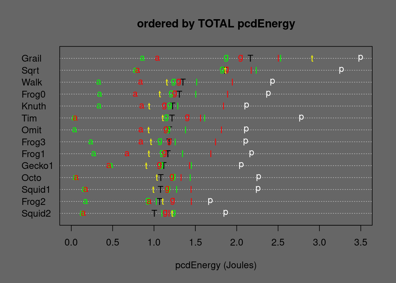
Figure 5.23: Medians of Mergesort alternatives ordered by TOTAL Energy. T=TOTAL, p=permut, t=tielog2; green: a=ascall, g=ascglobal, l=asclocal; red: a=descall, g=descglobal, l=desclocal

Figure 5.24: Medians of Mergesort alternatives ordered by TOTAL eFootprint. T=TOTAL, p=permut, t=tielog2; green: a=ascall, g=ascglobal, l=asclocal; red: a=descall, g=descglobal, l=desclocal
| r(%M) | r(rT) | r(pcdE) | r(pcdF) | d(pcdE) | p(rT) | p(pcdE) | p(pcdF) | |
|---|---|---|---|---|---|---|---|---|
| TOTAL | 0.57 | 0.81 | 0.82 | 0.47 | -0.22 | 0.0000 | 0.0000 | 0 |
| ascall | 0.57 | 0.38 | 0.38 | 0.22 | -0.21 | 0.0000 | 0.0000 | 0 |
| descall | 0.57 | 0.15 | 0.17 | 0.10 | -0.70 | 0.0000 | 0.0000 | 0 |
| ascglobal | 0.57 | 1.04 | 1.04 | 0.59 | 0.04 | 0.3595 | 0.4566 | 0 |
| descglobal | 0.57 | 1.00 | 1.01 | 0.58 | 0.01 | 0.1750 | 0.0023 | 0 |
| asclocal | 0.57 | 0.84 | 0.85 | 0.49 | -0.19 | 0.0000 | 0.0000 | 0 |
| desclocal | 0.57 | 0.64 | 0.64 | 0.37 | -0.66 | 0.0000 | 0.0000 | 0 |
| tielog2 | 0.57 | 1.30 | 1.30 | 0.74 | 0.28 | 0.0000 | 0.0000 | 0 |
| permut | 0.57 | 0.87 | 0.88 | 0.50 | -0.25 | 0.0000 | 0.0000 | 0 |
To illustrate the height of the greeNsort® Split&Merge inventions, I show the Innovation-lineage of Squidsort2: all innovations on which Squidsort2 depends form a (D)irected (A)cyclic (G)raph (DAG):
if (allinno)
  depplot(parents("Squidsort2"))
Figure 5.25: Innovation-lineage of Squidsort2
stability can be achieved by a workaround: using the positions as extra key, but that costs extra memory and more comparisons↩︎
Sebastian Wild (see Munro and Wild (2018)) has developed alternatives to Timsort with a drop-in replacement that are simpler and do an ‘optimized’ (more balanced) merging, but still based on an inefficient merge. The code for Peeksort and Powersort was not available at the time of running the simulations for this report, meanwhile I measured them, see Update: Powersort. Meanwhile O. R. L. Peters (2023a);O. R. L. Peters (2023b) seems to have improved the copy efficiency in his newest Glidesort, however that is Rust code and hence not measured here↩︎
For some implementations Timsort needs less than 50% buffer if no heavy merging is needed, for perfectly presorted data the buffer memory can be zero (
%RAM=1). In the Timsort code, %RAM is difficult to measure in a non-invasive way, therefore the test-bed assumes%RAM=1.5: the amount of memory that needs to be available to safely run Timsort↩︎the simpler Lazy-Funnelsort drops the contiguous Van-Emde-Boas memory layout↩︎