Chapter 4 Quicksort Algorithms
4.1 The Quicksort-Dilemma
I have described the greeNsort® resolution of the Quicksort-Dilemma in full length in the introductory chapter of the forthcoming greeNsort® book. I repeat this here in the short form typical for this disclosure.
The Quicksort1 algorithm of Hoare (1961a);Hoare (1961b) tried to be efficient (average \(\mathcal{O}(N\log{N})\)) and early-terminating on ties (\(\mathcal{O}(N\log{D})\)11), but on certain data inputs it degenerates to \(\mathcal{O}(N^2)\). Wrong implementations can even lead to endless loops \(\mathcal{O}(\infty)\), particularly when sentinels are used.
The popular Quicksort2 which goes back to Singleton (1969) and has been promoted by Sedgewick (1975);Sedgewick (1977b);Sedgewick (1977a);Sedgewick (1978) stops pointers on pivot-ties: this guarantees a balanced partitioning and hence an average \(\mathcal{O}(N\log{N})\), however it will not early-terminate on ties.

Figure 4.1: Quicksort2 compared to Quicksort2. The left chart compares the absolute energy consumed for 8 input patterns and the TOTAL (of 5). The right chart shows the respective ratios to the median of the reference algorithm (here Quicksort2). The red lines show the reference medians.
The also popular Quicksort3 developed by Bentley and McIlroy (1993) collects pivot-ties in a third partition between the low and high partition, this gives early termination but at the cost of extra operations and hence lower efficiency.
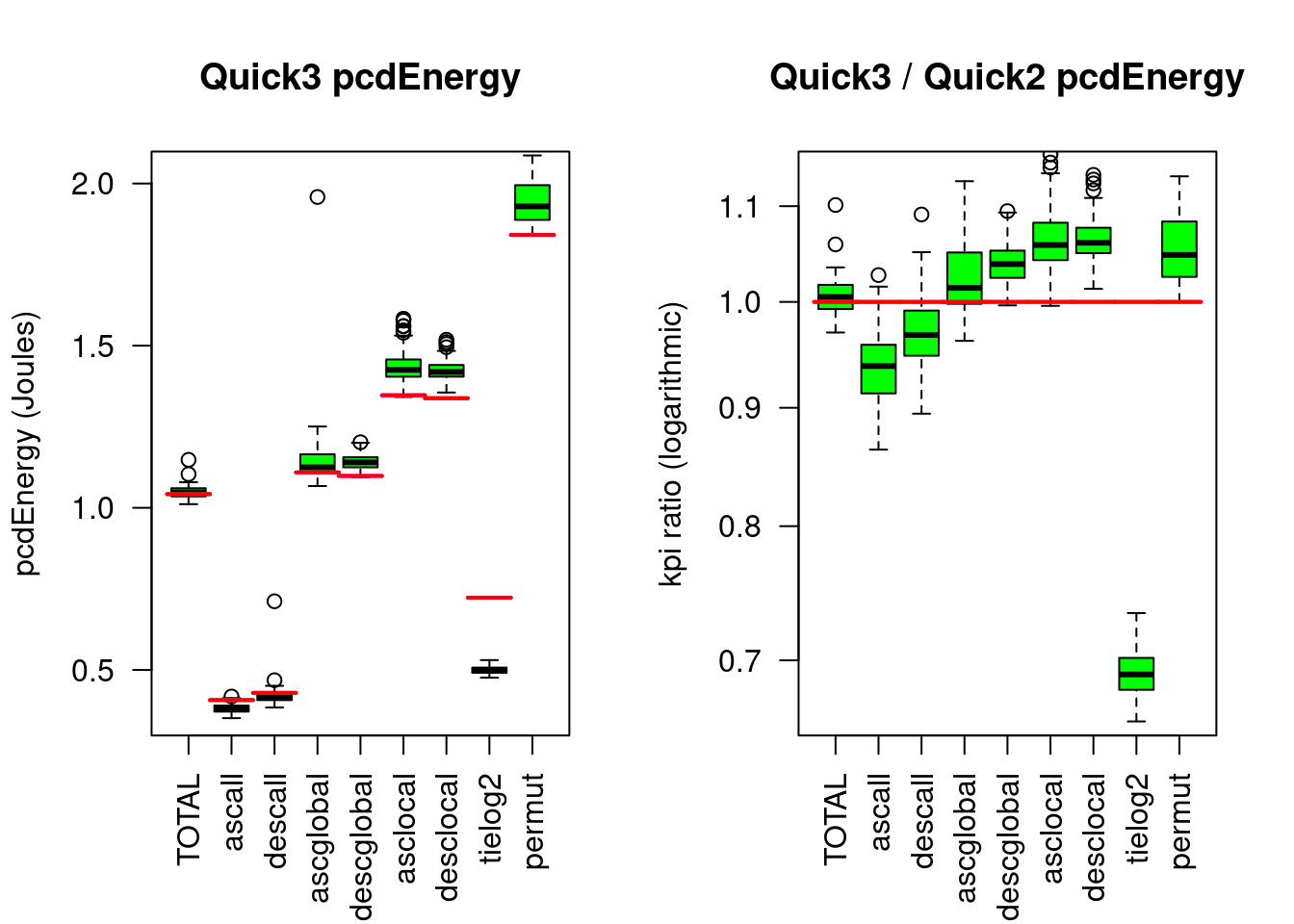
Figure 4.2: Quicksort3 compared to Quicksort2
The right chart shows less Energy consumption for the tied data (tielog2), but more Energy consumption for the hard sorting tasks such as completely random data (permut).
This is the Quicksort-Dilemma of the prior art: either you forego efficiency for non-tied data or you forego early termination on ties.
Here are some measurement results of for Quicksort2:
| %M | rT | pcdE | |
|---|---|---|---|
| TOTAL | 1 | 0.0870918 | 1.0424445 |
| ascall | 1 | 0.0314271 | 0.4071824 |
| descall | 1 | 0.0330232 | 0.4294158 |
| ascglobal | 1 | 0.0926678 | 1.1091954 |
| descglobal | 1 | 0.0929887 | 1.0982830 |
| asclocal | 1 | 0.1144985 | 1.3470172 |
| desclocal | 1 | 0.1147733 | 1.3378996 |
| tielog2 | 1 | 0.0588416 | 0.7229768 |
| permut | 1 | 0.1571141 | 1.8413511 |
And here Quicksort3 compared to Quicksort2 with results of conservative two-sided Wilcoxon tests:
| r(%M) | r(rT) | r(pcdE) | d(pcdE) | p(rT) | p(pcdE) | |
|---|---|---|---|---|---|---|
| TOTAL | 1 | 0.99 | 1.00 | 0.01 | 0.0000 | 0.0022 |
| ascall | 1 | 0.93 | 0.94 | -0.03 | 0.0000 | 0.0000 |
| descall | 1 | 0.97 | 0.97 | -0.01 | 0.0000 | 0.0000 |
| ascglobal | 1 | 1.00 | 1.01 | 0.02 | 0.4566 | 0.0056 |
| descglobal | 1 | 1.01 | 1.04 | 0.04 | 0.0000 | 0.0000 |
| asclocal | 1 | 1.05 | 1.06 | 0.08 | 0.0000 | 0.0000 |
| desclocal | 1 | 1.04 | 1.06 | 0.08 | 0.0000 | 0.0000 |
| tielog2 | 1 | 0.65 | 0.69 | -0.22 | 0.0000 | 0.0000 |
| permut | 1 | 1.04 | 1.05 | 0.09 | 0.0000 | 0.0000 |
Compared to Quicksort2, Quicksort3 needs only 68% Energy on strongly tied data, but without a TOTAL benefit, because it needs 4% more Energy on randomly permuted data.
Recent attempts to solve the Quicksort-Dilemma lead to significant improvements but still not to algorithmically convincing solutions:
- Yaroslavskiy (2009) published the dual-pivot Quicksort (Dupisort) used such extra-operations to create a real third partition, this improves the average \(\mathcal{O}(N\log_2{N})\) algorithm to \(\mathcal{O}(N\log_3{N})\) regarding moves, but the algorithm is strongly serial and difficult to implement branchless. greeNsort® slightly improved the algorithm by removing a redundant branch (Tricksort).
- Edelkamp and Weiß (2016),Edelkamp and Weiss (2016) published the much faster and simpler Block-Quicksort (see Quicksort2B), but only with a rudimentary and expensive early-termination mechanism12.
- O. Peters (2014);O. Peters (2015);O. R. L. Peters (2021b) combined a branchless algorithm with a proper tuning for ties and a proper tuning for presorted data, the tuning overhead of extra operations in his Pattern-Defeating Quicksort (Pdqsort) is very little, so it is close to optimal, see the excellent C++ implementation on github. However, instead of being algorithmically clean, Pdqsort uses some heuristic shuffling. Furthermore, the fallback to Heapsort can slow down performance (see O. R. L. Peters (2021a)), and once combined with an expensive comparison function such as localized string comparison
strcoll, it becomes slower than Quicksort2.
4.2 greeNsort® solution
The mentioned approaches of the prior art share that they attempt to achieve symmetry on the loop-level, which contradicts the greeNsort® Symmetric-asymmetry principle. Asymmetric-partitioning on the loop level has been banned by Sedgewick (1977a):
Program 3, due to its asymmetrical nature, can produce unbalanced partitions […] unary files represent the worst case for Program 3 […] Program 3 is also quadratic for binary files […] The evidence in favor of stopping the scanning pointers on keys equal to the partitioning element in Quicksort is overwhelming — Sedgewick (1977)
This was the point in history where Quicksort2 became standard, until Quicksort3 was engineered and declared “optimal” by Sedgewick and Bentley (2002). It is time to revise these decisions now.
4.2.1 DIET method
innovation("MECEP","T*","MECEP partitioning")
dependency("MECEP","Partition&Pool")
innovation("No3rd-partition","C","Early Termination without 3rd partition")
innovation("Asymmetric-partitioning","C","Asymmetric-partitioning is good")
dependency("Asymmetric-partitioning","MECEP")
innovation("DIET","B","Distinct Identification for Early Termination")
dependency("DIET","No3rd-partition")
dependency("DIET","Asymmetric-partitioning")
dependency("DIET","NORELORE")
First I drop the prior art assumption, that early-termination on ties requires collecting pivot-ties in a third (middle) partition. Early-termination on ties not even needs two partitions. An algorithm can early-terminate in a single partition. Once the algorithm knows that one partition is purely composed of pivot-ties (Sedgewick’s ‘unary files’) it can stop further partitioning and recursion. QED. So far this early-termination works only for a special simple case, but simplicity wins. How can this generalized to early terminate for multiple distinct tied values? By using T-level technique - (M)utually (E)xclusive and (C)ollectively (E)xaustive (P))artitioning (MECEP). QED. As an example consider a file with four distinct values: a binary MECEP can result in two files with two distinct values each, after another recursion it is possible to have four unary files and early-terminate. How does one do MECE binary partitioning? By revising Sedgewick’s ban on Asymmetric-partitioning: all pivot-ties go to one side. How can unary files be identified efficiently? By applying the T-level technique – (NO)-(RE)gret (LO)op-(RE)use (NORELORE) principle. In Asymmetric-partitioning, one pointer search contains equality (LE or GE) the other not (LT or GT), if the first pointer search runs while(EQ(x[i],pivot) and continues with while(LE(x[i],pivot) or while(GE(x[i],pivot), then it is possible to identify unary files at almost no extra cost: the algorithm simply starts with a no-regret pre-loop while(EQ(x[i],pivot). If this pre-loop reaches the other side the algorithm knows to have a unary file and can early terminate. If this pre-loop finds a key that is different from the pivot, then no work has been wasted because the same decision was made as if the first pointer search of the main loop had been used. That is, the result of this pre-loop can be re-used. Only for the last key different from the pivot the query needs to find out whether this element belongs to the same or the other partition. This implies that instead of \(N-1\) comparisons for binary partitioning only one single extra comparison is needed to identify unary files. I call this the B-level innovation – (D)istinct (I)dentification for (E)arly (T)ermination (DIET) method. Since with \(N-1\) comparisons it is not possible to binary partition and identify unary input, with only one more comparison DIET is optimal. QED.
4.2.2 Engineering Zocksort
innovation("Zocksort","A", "self-recursive DIET Quicksort")
dependency("Zocksort", "DIET")
Coding the DIET-method into a prior art self-recursion function gives an optimal early terminating Quicksort (named Zocksort) with an Achilles heel. For example, if the Asymmetric-partitioning is defined as
| left partition | right partition |
|---|---|
LE(x[i], pivot) |
GT(x[i], pivot) |
111011111111111 |
`` |
then having input data composed of one 0 and many 1’s is likely to sample 1 as a pivot and partition all values into the left partition. Only if 0 is sampled as the pivot, 0 and 1’s are separated into two partitions. This implies an expected \(\mathcal{O}(N^2)\) worst case. The risky word ‘Zock’ comes from German ‘zocken’ which means ‘gambling’ and is a onomatopoeia resembling smashing cards on the table.
4.2.3 FLIP method
innovation("FLIP","B","Fast Loops In Partitioning")
dependency("FLIP","Asymmetric-partitioning")
dependency("FLIP","Symmetric-recursion")
Because of this asymmetric risk Sedgewick (1977a) condemned Asymmetric-partitioning. Instead of fighting asymmetric loops, greeNsort® embraces them and delegates symmetry-creation to T-level technique - (COM)puting on the (REC)ursion (COMREC). Instead of self-recursion, which perpetuates asymmetry, greeNsort® uses Symmetric-recursion. Note that any input data that can fool the above Asymmetric-partitioning, cannot fool the left-right-mirrored Asymmetric-partitioning:
| left partition | right partition |
|---|---|
LT(x[i], pivot) |
GE(x[i], pivot) |
0 |
11111111111111 |
Mutually recursing between those two mirrored Asymmetric-partitioning functions prevents being fooled by any asymmetric input data. QED. I name this the B-level innovation – (F)ast (L)oops (I)n (P)artitioning (FLIP) method. FLIP is an acronym and a mnemonic for mirroring.
4.2.4 Engineering Zacksort
innovation("Zacksort","A", "zig-zagging DIET-FLIP Quicksort")
dependency("Zacksort", "DIET")
dependency("Zacksort", "FLIP")
Figure 4.3: Zacksort zig-zagging symmetric recursion
One way to combine the DIET with the FLIP method is zig-zagging between putting pivot-ties into the left partition on one recursion-level and into the right partition on the next recursion-level. The mutual-recursion is: the left function calls the right function in left and right branches, the right function calls the left function in the left and right branch. The German translation of zig-zag is ‘Zick-Zack’ and ‘Zack’ also means ‘quick’, hence the name Zacksort.

Figure 4.4: Zacksort compared to Quicksort3
| r(%M) | r(rT) | r(pcdE) | d(pcdE) | p(rT) | p(pcdE) | |
|---|---|---|---|---|---|---|
| TOTAL | 1 | 0.99 | 0.99 | -0.01 | 0e+00 | 0.0000 |
| ascall | 1 | 0.99 | 0.99 | 0.00 | 3e-04 | 0.0034 |
| descall | 1 | 0.97 | 0.98 | -0.01 | 0e+00 | 0.0000 |
| ascglobal | 1 | 1.03 | 1.04 | 0.04 | 0e+00 | 0.0000 |
| descglobal | 1 | 1.03 | 1.03 | 0.03 | 0e+00 | 0.0000 |
| asclocal | 1 | 1.03 | 1.02 | 0.03 | 0e+00 | 0.0000 |
| desclocal | 1 | 1.02 | 1.02 | 0.03 | 0e+00 | 0.0000 |
| tielog2 | 1 | 0.66 | 0.66 | -0.25 | 0e+00 | 0.0000 |
| permut | 1 | 1.03 | 1.02 | 0.03 | 0e+00 | 0.0002 |
Compared to Quicksort2, Zacksort needs only 99% Energy, due to 66% Energy on strongly tied data. Remember, that Quicksort3 needed in TOTAL more Energy than Quicksort2.
4.2.5 Engineering Zucksort
innovation("Zucksort","A", "semi-flipping DIET-FLIP Quicksort")
dependency("Zucksort", "DIET")
dependency("Zucksort", "FLIP")
Figure 4.5: Zucksort semi-flipping symmetric recursion, red branches can have pivot-ties
Another way to combine DIET and FLIP is flipping the pivot-asymmetry only in that branch, that can contain pivot-ties, the other branch is not at risk for quadratic execution costs. Assume the left function puts pivot-ties left and the right function puts pivot-ties right, then the mutual-recursion is: the left function flips to calling the right function on the left branch and keeps calling the left function on the right branch; while the right function keeps calling the right function on the left branch and flips to calling the left function on the right branch.
4.2.6 POET method
innovation("POET","B", "Pre-Order Early Termination")
dependency("POET", "NORELORE")
So far Zucksort early terminates only on ties, not on presorted data. Testing in a loop for presorted data before starting to sort is not new, and is an extra-investment of comparisons which may or may not pay-off. I now present the POET method, which like the DIET-method employs the NORELORE principle as much as possible. The initial idea of POET was to put a second pre-loop between the DIET-loop and the MAIN-loop such that - without regret - each loop spills into the next and the next leverages the work done so far by the previous. Let’s see: Once the DIET-loop terminates without early-termination, the last inspected element is distinct from the pivot, but still can be presorted relative to the previous element (or be the first element). I.E. it is possible to continue with a POET-loop with only one comparison overlap. The POET-loop either reaches the other side, confirming completely presorted data and results in early-termination, or it breaks and needs to be followed by the MAIN loop. So far the theory. In practice, there are a couple of difficulties:
- the initial SWAP for placing the pivot at the beginning of the data is incompatible with presorted data, hence must not be done
- without the SWAP the DIET loop needs to compare one more element
- reading the pivot before and doing this SWAP after the POET loop costs two large-distance operations
- not knowing the position of the pivot after partitioning does not allow to exclude it between the left and right partition, which (theoretically) gives a \(\mathcal{O}(\infty)\) instead of a \(\mathcal{O}(N^2)\) worst case
- reusing the progress of a break-ed POET loop is not trivial, theoretically one could identify the first element of the presorted sequence that belongs to the other partition by binary search and then enter a (B)inary (I)dentified (A)symmetric (S)earch (BIAS)-loop. A BIAS-loop could simply increment the pointer along the presorted sequence and search only on the other side for elements that need swapping, this is theoretically cheaper than the final MAIN-loop, which needs to compare on both sides.
In summary: the idea to put a POET-loop between the DIET-loop and the MAIN-loop is still to complicated, violates the DONOTUBE principle and does not pay-off. The POET method is actually much simpler: instead the POET-loop simply replaces the DIET-loop. This is possible, because an all-tied sequence formally is presorted, hence a POET-loop having affirmed complete presortedness enables early-termination for all-tied data. Different from the DIET-loop, the progress of the POET-loop cannot be reused by the MAIN-loop, hence, misinvested comparisons are lost and the MAIN-loop needs to start from scratch. This is less dramatic than it sounds. Yes, the DIET-method was provably optimal with at most one misinvested comparison per partitioning (deterministically) and the POET-method does not have this property. But under random input the expected number of misinvested comparisons is smaller-equal one. And any non-random non-presorted data that lures the algorithm into big progress of the POET-loop must be highly structured, and hence is likely to be early terminated in its branches.
4.2.7 Engineering Ducksort
innovation("Ducksort","A", "semi-flipping POET-FLIP Zucksort")
dependency("Ducksort", "Zucksort")
dependency("Ducksort", "POET")
The resulting algorithm of replacing the DIET-method with the B-level innovation – (P)re-(O)rder (E)arly (T)ermination (POET)-method in Zucksort is called Ducksort and the differences are:
| Zucksort | Ducksort |
|---|---|
| 1. delegate to Insertionsort if small | 1. delegate to Insertionsort if small |
| 2. sample pivot and SWAP as sentinel | 2. POET-loop potentially early terminates |
| 3. DIET-loop potentially early terminates | 3. sample pivot and SWAP as sentinel |
| 4. otherwise MAIN-loop | 4. otherwise MAIN-loop |
| 5. SWAP pivot into position | 5. SWAP pivot into position |
| 6. recall left and right excluding pivot | 6. recall left and right excluding pivot |
The simplicity of Ducksort is almost poetically beautiful! A few lines of code and mirroring them is clearly superior to the famous Quicksort3: Ducksort early-terminates on more best-cases and still is faster on random input. Furthermore it can be block-tuned (DucksortB) which is difficult with Quicksort3. Note finally that Ducksort can further be tuned to also early-terminate on slightly disturbed presorted data, using the limited Insertionsort from Pdqsort (see O. Peters (2014);O. Peters (2015);O. R. L. Peters (2021b)). I have tried this, but did not find such ordinary tuning-trade-offs convincing (NORELORE).
Despite all the enthusiasm about the elegance of Ducksort, it should not be concealed that the practical benefit of the additional adaptivity is limited: theoretically, every branch in the recursion can recognize presorted data, but in practice this hardly ever happens: when the recursion has zoomed into a presorted area with partially presorted data, the formerly presorted data has long since been scrambled by the previous partitioning SWAPs. Truly effective processing of presorted data is the domain of Split&Merge Algorithms. An alternative to achieve \(\mathcal{O}(N)\) for completely presorted data is to simply use a single POET-loop before recursion begins (named ZucksortA in the test-bed).
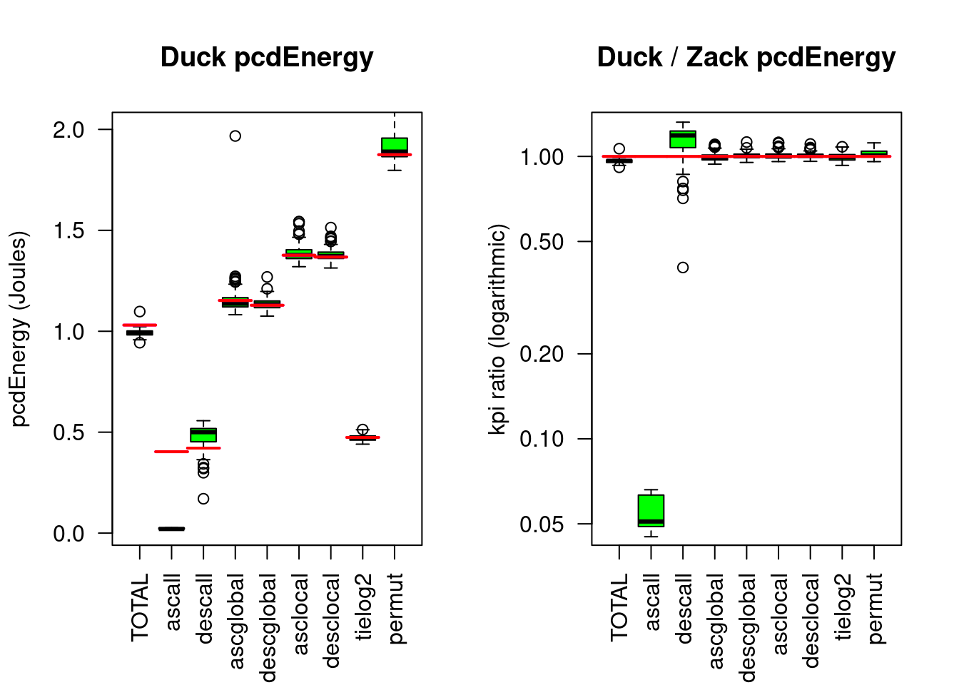
Figure 4.6: Ducksort compared to Zacksort
| r(%M) | r(rT) | r(pcdE) | d(pcdE) | p(rT) | p(pcdE) | |
|---|---|---|---|---|---|---|
| TOTAL | 1 | 0.96 | 0.96 | -0.04 | 0.0000 | 0.0000 |
| ascall | 1 | 0.05 | 0.05 | -0.38 | 0.0000 | 0.0000 |
| descall | 1 | 1.20 | 1.19 | 0.08 | 0.0000 | 0.0000 |
| ascglobal | 1 | 0.99 | 0.99 | -0.02 | 0.0000 | 0.0891 |
| descglobal | 1 | 0.99 | 1.00 | 0.01 | 0.0000 | 0.2645 |
| asclocal | 1 | 0.99 | 1.00 | 0.00 | 0.0000 | 0.8298 |
| desclocal | 1 | 0.99 | 1.00 | 0.01 | 0.0003 | 0.0865 |
| tielog2 | 1 | 0.99 | 0.99 | 0.00 | 0.1482 | 0.2039 |
| permut | 1 | 1.00 | 1.01 | 0.02 | 0.6096 | 0.1602 |
Compared to Zacksort, Ducksort needs only 96% Energy due to only 5% Energy on presorted data.
4.2.8 Partial Z:cksort
innovation("Zackpart","F", "MECEP partial sorting between l and r")
innovation("Zuckpart","F", "MECEP partial sorting between l and r")
dependency("Zackpart", "Zacksort")
dependency("Zuckpart", "Zucksort")
innovation("Zackselect","F", "MECEP more informative than Quickselect")
innovation("Zuckselect","F", "MECEP more informative than Quickselect")
dependency("Zackselect", "Zackpart")
dependency("Zuckselect", "Zuckpart")
innovation("Zackpartleft","F", "MECEP partial sorting left of r")
innovation("Zuckpartleft","F", "MECEP partial sorting left of r")
dependency("Zackpartleft", "Zackpart")
dependency("Zuckpartleft", "Zuckpart")
innovation("Zackpartright","F", "MECEP partial sorting right of l")
innovation("Zuckpartright","F", "MECEP partial sorting right of l")
dependency("Zackpartright", "Zackpart")
dependency("Zuckpartright", "Zuckpart")
From Quicksort1 Hoare (1961a);Hoare (1961c) derived the ‘FIND’ algorithm, later known as Quickselect. Quickselect is a special case of partial sorting (Quickpart). Let \(X\) be an unsorted set of \(N\) elements and \(Y\) the sorted version of this set. Quickpart (usually following the logic of Quicksort2) takes as input \(X\) and two positions \(l,r\) where \(1 \le l,r \le N\) and returns a partially sorted set \(Z\) such that
\[ \begin{array}{rcl} Z[i<l] & \le & Y[l] \\ Z[l..r] & = & Y[l..r] \\ Z[i>r] & \ge & Y[r] \end{array}\]
Note the use of \(\le\) and \(\ge\) because ties can go to both partitions. Let ‘Z:ck’ denote both, ‘Zack’ and ‘Zuck’, then designing Z:ckpart following the logic of Z:cksort gives similar algorithms but due to MECEP with stricter guarantees:
\[ \begin{array}{rcl} Z[i<l] & < & Y[l] \\ Z[l..r] & = & Y[l..r] \\ Z[i>r] & > & Y[r] \end{array}\]
Different constraints on the parameters \(l\) and \(r\) give special case-algorithms:
| prior art | greeNsort | constraints on l,r |
|---|---|---|
| Quickpart | Z:ckpart | (none) |
| Quickpartleft | Z:ckpartleft | l=1 |
| Quickpartright | Z:ckpartright | r=N |
| Quicksort | Z:cksort | l=1, r=N |
| Quickselect | Z:ckselect | l=r |
The difference between the prior art and the greeNsort® algorithms is best demonstrated by comparing Quickselect and Z:ckselect. The former ignores ties and the only meaningful return-value is the key-value at position \(l=r\). The latter returns the positions of the leftmost and rightmost ties to that value, hence is more informative: we learn whether the data is tied at this position and how much it is tied. In Quickselect, ties to \(Y[l=r]\) can be anywhere, Z:ckselect guarantees that all ties are in the position where they would be in the fully sorted set \(Y\), hence Z:ckselect does somewhat more sorting work:
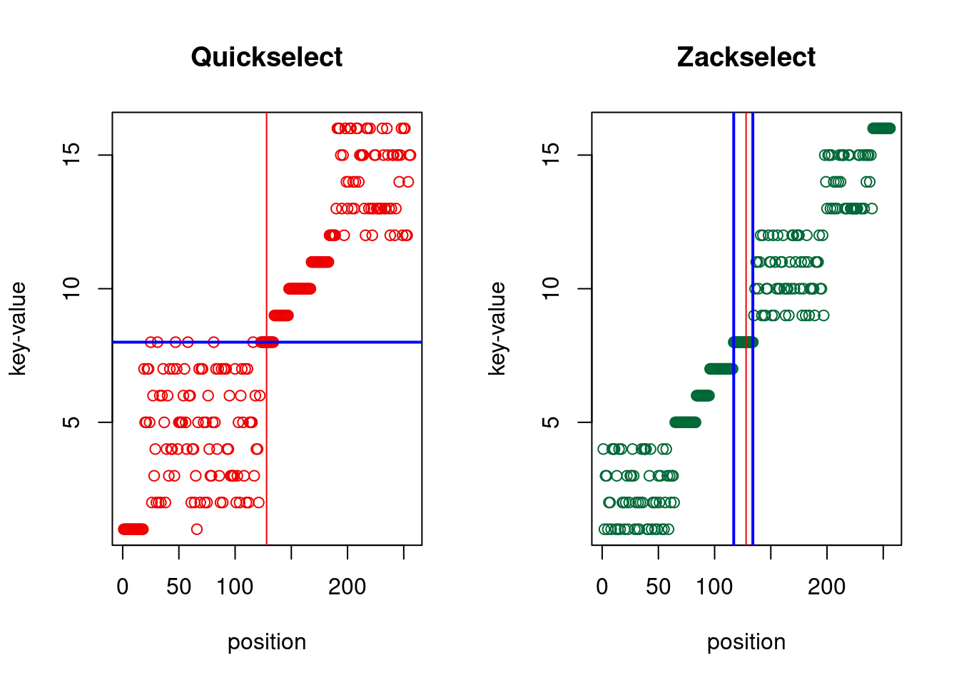
Figure 4.7: Quickselect versus Zackselect, return value(s) in blue
The cost of both is comparable and both have expected \(\mathcal{O}(N)\).
4.2.9 Z:cksort implementation
When using random pivots, Z:cksort has expected \(\mathcal{O}(N \log{D})\) cost for \(D\) distinct keys due to ties. This probabilistic guarantee of \(\mathcal{O}(N \log{N})\) or better is lost when using deterministic pivots such as median-of-three. Replacing a random pivot by an assumption about random data (Sedgewick:1977a) is academic and dangerous:
The first principle was security […] logically impossible for any source language program to cause the computer to run wild, either at compile time or at run time. […] I note with fear and horror that even in 1980, language designers and users have not learned this lesson. In any respectable branch of engineering, failure to observe such elementary precautions would have long been against the law. — Tony Hoare (The 1980 ACM Turing Award Lecture)
Yes, using random number generators in Quicksorts and Z:cksorts has a cost which can be saved, but a proper deterministic implementation must control recursion depth and fall back to an algorithm with \(\mathcal{O}(N \log{N})\) guarantees. Note that falling back to Heapsort as in Introsort comes with a performance hit13. When implementing Z:cksort with deterministic pivots, the same pivots should be selected in the left and right version of the algorithm (hence not perfectly symmetric): this guarantees that a misbehaved pivot will be rendered harmless at the next recursion level. Z:cksort is quite well-behaved when taking a pivot from the middle, however it remains attackable, hence serious code using deterministic pivots must implement a fallback. Note that the most efficient fallback is Z:cksort with random pivots: the expected execution cost is always \(\mathcal{O}(N \log{N})\) and RUNtime about factor 3 better than Heapsort, hence it is never rational to switch to Heapsort (unless probabilistic behavior is fundamentally unacceptable in the given context).
Like Quicksort2, Z:cksort can be implemented with sentinels14 and block-tuned (see ZacksortB, ZucksortB and DucksortB) as predicted by Hoare (1962) and rediscovered by Edelkamp and Weiß (2016),Edelkamp and Weiss (2016).
Quicksort2 can be easily executed in parallel branches (PQuicksort2, PQuicksort2B), however, parallel partitioning is complicated. The same is true for Z:cksort (PDucksort, PDucksortB).
4.3 Quicksort conclusion
I have shown how the Quicksort-Dilemma can be resolved and how exactly that symmetric probabilistic algorithm can be written which Tony Hoare tried to design with Quicksort1. Tony Hoare was almost successful, but the challenges of the ‘almost’ persisted for 60 years. I have shown that the prior art took a wrong turn in the seventies where it condemned Asymmetric-partitioning loops, which then was followed by many subsequent failures. Zacksort and Zucksort are elegant solutions that combine efficiency with early termination on tied data, and Ducksort additionally achieves early termination on presorted data without increasing code-complexity. This use of symmetry seamlessly leads to partial sorting algorithms that consistently handle ties and return more useful information.

Figure 4.8: Medians of Quicksort alternatives ordered by TOTAL Energy. T=TOTAL, p=permut, t=tielog2; green: a=ascall, g=ascglobal, l=asclocal; red: a=descall, g=descglobal, l=desclocal
| r(%M) | r(rT) | r(pcdE) | d(pcdE) | p(rT) | p(pcdE) | |
|---|---|---|---|---|---|---|
| TOTAL | 1 | 0.95 | 0.95 | -0.05 | 0 | 0 |
| ascall | 1 | 0.05 | 0.05 | -0.39 | 0 | 0 |
| descall | 1 | 1.17 | 1.16 | 0.07 | 0 | 0 |
| ascglobal | 1 | 1.02 | 1.02 | 0.03 | 0 | 0 |
| descglobal | 1 | 1.02 | 1.03 | 0.04 | 0 | 0 |
| asclocal | 1 | 1.02 | 1.02 | 0.03 | 0 | 0 |
| desclocal | 1 | 1.02 | 1.03 | 0.03 | 0 | 0 |
| tielog2 | 1 | 0.66 | 0.65 | -0.25 | 0 | 0 |
| permut | 1 | 1.02 | 1.03 | 0.05 | 0 | 0 |
| r(%M) | r(rT) | r(pcdE) | d(pcdE) | p(rT) | p(pcdE) | |
|---|---|---|---|---|---|---|
| TOTAL | 1 | 0.87 | 0.87 | -0.13 | 0e+00 | 0.0000 |
| ascall | 1 | 0.03 | 0.04 | -0.59 | 0e+00 | 0.0000 |
| descall | 1 | 1.05 | 1.06 | 0.04 | 0e+00 | 0.0000 |
| ascglobal | 1 | 0.98 | 0.99 | -0.01 | 0e+00 | 0.0118 |
| descglobal | 1 | 0.98 | 0.99 | -0.01 | 0e+00 | 0.0004 |
| asclocal | 1 | 0.99 | 1.00 | 0.00 | 0e+00 | 0.4608 |
| desclocal | 1 | 0.99 | 0.99 | -0.01 | 0e+00 | 0.0019 |
| tielog2 | 1 | 0.36 | 0.39 | -0.41 | 0e+00 | 0.0000 |
| permut | 1 | 0.99 | 1.01 | 0.01 | 4e-04 | 0.0570 |
Ducksort saves 5% Energy compared to Quicksort2, comparing the block-tuned versions the savings are even 13% (due to saving 64% on strongly tied data).
To illustrate the height of the greeNsort® inventions after this entrenched tradition of mistaken historical development, here is the Innovation-lineage of Ducksort: all innovations on which Ducksort depends form a (D)irected (A)cyclic (G)raph (DAG):
Figure 4.9: Innovation-lineage of Ducksort
where \(D\) is the number of Distinct keys↩︎
Fun fact: the optimization published by Edelkamp&Weiß (2016) was already suggested in a little known paper of Hoare (1962) in which he gives context and explanations for his 1961 algorithm↩︎
about factor 3 slower, or worse in case of ties↩︎
the greeNsort® implementations use the pivot as sentinel one one side, both-sided sentinels are also possible albeit with less elegant code↩︎